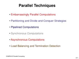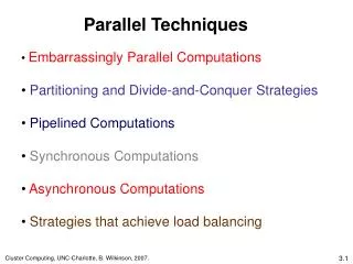
Embarrassingly Parallel Computations Chapter 3
This chapter explores the concept of embarrassingly parallel computations, which can be easily divided into independent tasks that require minimal communication between processes. We examine practical applications, including low-level image processing, the Mandelbrot set, and Monte Carlo calculations. This text further delves into computation techniques like static and dynamic task assignments, demonstrating how to efficiently parallelize computational tasks, especially in scenarios like generating area estimates or calculating π.

Embarrassingly Parallel Computations Chapter 3
E N D
Presentation Transcript
Embarrassingly Parallel Computations Chapter 3
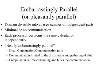
Embarrassingly Parallel Computations A computation that can obviously be divided into a number of completely independent parts, each of which can be executed by a separate process. No communication or very little communication between processes Each process can do its tasks without any interaction with others
Practical embarrassingly parallel computation (static process creation / master-slave approach)
Embarrassingly Parallel Computations • Examples • Low level image processing • Many of such operations only involve local data with very limited if any communication between areas of interest. • Mandelbrot set • Monte Carlo Calculations
Some geometrical operations Shifting Object shifted by Dxin the x-dimension and Dyin the y-dimension: x¢ = x + Dx y¢ = y + Dy where x and y are the original and x¢ and y¢ are the new coordinates. Scaling Object scaled by a factor Sxin x-direction and Syin y-direction: x¢ = xSx y¢ = ySy Rotation Object rotated through an angle q about the origin of the coordinate system: x¢ = x cosq + y sinq y¢ = -x sinq + y cosq
Partitioning into regions for individual processes Square region for each process (can also use strips)
Mandelbrot Set What is the Mandelbrot set? Set of all complex numbers c for which sequence defined by the following iterationremains bounded: z(0) = c, z(n+1) = z(n)*z(n) + c, n=0,1,2, ... This means that there is a number B such that the absolute value of all iterates z(n) never gets larger than B.
Sequential routine computing value of one point • structure complex { • float real; • float imag; • }; • intcal_pixel(complex c) • { int count, max; • complex z; • float temp, lengthsq; • max = 256; • z.real = 0; z.imag = 0; • count = 0; /* number of iterations */ • do { • temp = z.real * z.real - z.imag * z.imag + c.real; • z.imag = 2 * z.real * z.imag + c.imag; • z.real = temp; • lengthsq = z.real * z.real + z.imag * z.imag; • count++; • } while ((lengthsq < 4.0) && (count < max)); • return count; • }
Parallelizing Mandelbrot Set Computation Static Task Assignment Simply divide the region into fixed number of parts, each computed by a separate processor. Disadvantage: Different regions may require different numbers of iterations and time. Dynamic Task Assignment
Monte Carlo Methods • Another embarrassingly parallel computation • Example: • calculate πusing the ratio: • Randomly choose points within the square • Count the points that lie within the circle • Given a sufficient number of randomly selected samples • fraction of points within the circle will be: π /4
Example of Monte Carlo Method Area = D2
Computing an Integral Use random values of x to compute f(x) and sum values of f(x): where xiare randomly generated values of x between x1 and x2. Monte Carlo method is very useful if the function cannot be integrated numerically (maybe having a large number of variables)
Example: Sequential Code sum = 0; for (i = 0; i < N; i++) { /* N random samples */ xr = rand_v(x1, x2); /* generate next random value */ sum = sum + xr * xr - 3 * xr; /* compute f(xr) */ } area = (sum / N) * (x2 - x1); Routine rand_v(x1, x2) returns a pseudorandom number between x1 and x2
Values for a "good" generator: a=16807, m=231-1 (a prime number), c=0 This generates a repeating sequence of (231- 2) different numbers.
A Parallel Formulation xi+1 = (axi + c) mod m xi+k = (Axi+ C) mod m A and C above can be derived by computing xi+1=f(xi) , xi+2=f(f(xi)), ... xi+k=f(f(f(…f(xi)))) and using the following properties: • (A+B) mod M = [(A mod M) + (B mod M)] mod M • [ X(A mod M) ] mod M = (X.A mod M) • X(A + B) mod M = (X.A + X.B) mod M = [(X.A mod M) + (X.B mod M)] mod M • [ X( (A+B) mod M) ] mod M = (X.A + X.B) mod M