Download
1 / 28
280 likes | 298 Vues
Explore cache principles, design behaviors, and placement schemes to enhance system speed and efficiency. Learn about direct-mapped, fully-associative, and set-associative cache strategies. Gain insights into cache performance formulas and memory hierarchy concepts.

E N D
Introduction • Cache ABCs • Cache Performance • Write policy • Virtual Memory and TLB Appendix B. Review of Memory Hierarchy • CDA5155 Fall 2013, Peir / University of Florida
Cache Basics • A cache is a (hardware managed) storage, intermediate in size, speed, and cost-per-bit between the programmer-visible registers (usually SRAM) and main physical memory (usually DRAM), used to hide memory latency • The cache itself may be SRAM or fast DRAM. • There may be >1 levels of caches • Basis for cache to work: Principle of Locality • When a location is accessed, it and “nearby” locations are likely to be accessed again soon. • “Temporal” locality - Same location likely again soon. • “Spatial” locality - Nearby locations likely soon.
Cache Performance Formulas • Memory stalls per program (blocking cache): • CPU time formula: • More cache performance will be given later!
Four Basic Questions • Consider access of levels in a memory hierarchy. • For memory: byte addressable • For caches: Use block (or called line) for the unit of data transfer; satisfy Principle of Locality. But, need to locate blocks (not byte addressable) • Transfer between cache levels, and the memory • Cache design is described by four behaviors: • Block Placement: • Where could a new block be placed in the level? • Block Identification: • How is a block found if it is in the level? • Block Replacement: • Which existing block should be replaced if necessary? • Write Strategy: • How are writes to the block handled?
Direct-Mapped Placement • A block can only go into one frame in the cache • Determined by block’s address (in memory space) • Frame number usually given by some low-order bits of block address. • This can also be expressed as: • (Frame number) = (Block address) mod (Number of frames (sets) in cache) • Note that in a direct-mapped cache, • block placement & replacement are both completely determined by the address of the new block that is to be accessed.
Direct-Mapped Identification • Tags • Block frames • Tags for locating block • Memory Address • Block Data • Frm# • Tag • Off. • Decode & Row Select • One Selected &Compared • Muxselect • ? • Compare Tags • Data Word • Hit
Fully-Associative Placement • One alternative to direct-mapped is: • Allow block to fill any empty frame in the cache. • How do we then locate the block later? • Can associate each stored block with a tag • Identifies the block’s location in cache. • When the block is needed, we can use the cache as an associative memory, using the tag to match all frames in parallel, to pull out the appropriate block. • Another alternative to direct-mapped is placement under full program control. • A register file can be viewed as a small programmer-controlled cache (w. 1-word blocks).
Fully-Associative Identification • Block addrs • Block frames • Address • Block addr • Off. • Parallel Compare& Select • Note that, compared to Direct-M: • More address bits have to be stored with each block frame. • A comparator is needed for each frame, to do the parallel associative lookup. • Muxselect • Hit • Data Word
Set-Associative Placement • The block address determines not a single frame, but a frame set (several frames, grouped together). • (Frame set #) = (Block address) mod (# of frame sets) • The block can be placed associatively anywhere within that frame set. • If there are n frames in each frame set, the scheme is called “n-way set-associative”. • Direct mapped = 1-way set-associative. • Fully associative: There is only 1 frame set.
Set-Associative Identification • Tags • Block frames • Address • Set# • Tag • Off. • Note:4separatesets • Set Select • Parallel Compare within the Set • Intermediate between direct-mapped and fully-associative in number of tag bits needed to be associated with cache frames. • Still need a comparator for each frame (but only those in one set need be activated). • Muxselect • Hit • Data Word
Cache Size Equation • Simple equation for the size of a cache: • (Cache size) = (Block size) × (Number of sets) × (Set Associativity) • Can relate to the size of various address fields: • (Block size) = 2(# of offset bits) • (Number of sets) = 2(# of index bits) • (# of tag bits) = (# of memory address bits) (# of index bits) (# of offset bits) • Determine the set • Memory address
Replacement Strategies • Which block do we replace when a new block comes in (on cache miss)? • Direct-mapped: There’s only one choice! • Associative (fully- or set-): • If any frame in the set is empty, pick one of those. • Otherwise, there are many possible strategies: • (Pseudo-) Random: Simple, fast, and fairly effective • Least-Recently Used (LRU),and approximations thereof • Require bits to record replacement info., e.g. 4-way requires 4! = 24 permutations, need 5 bits to define the MRU to LRU positions • Least-Frequently Used (LFU) using counters • Optimal: Replace the block used farthest future (possible?)
Implement LRU Replacement • Pure LRU, 4-way use 6 bits (minimum 5 bits) • Partitioned LRU (Pseudo LRU): • Instead of record full combination, use a binary tree to maintain only (n-1) bits for n-way set associativity • 4-way example: • 13 • 23 • 24 • 34 • 12 • 14 • 0 • 01 • 0 • 0 • 1 • 10 • LRU • LRU • LRU • Replacement
Write Strategies • Most accesses are reads, not writes • Especially if instruction reads are included • Optimize for reads – What matters performance • Direct mapped can return value before valid check • Writes are more difficult • Can’t write to cache till we know the right block • Object written may have various sizes (1-8 bytes) • When to synchronize cache with memory? • Write through - Write to cache & to memory • Prone to stalls due to high bandwidth requirements • Write back - Write to memory upon replacement • Memory may be out of date
Write Miss Strategies • What do we do on a write to a block that’s not in the cache? • Two main strategies: Both do not stop processor • Write-allocate (fetch on write) - Cache the block. • No write-allocate (write around) - Just write to memory. • Write-back caches tend to use write-allocate. • White-through tends to use no write-allocate. • Use Dirty Bit to indicate writeback is needed in write-back strategy • Remember, write won’t occur until commit (out-of-order model)
Write Buffers • A mechanism to help reduce write stalls • On a write to memory, block address and data to be written are placed in a write buffer. • CPU can continue immediately • Unless the write buffer is full. • Write merging: • If the same block is written again before it has been flushed to memory, old contents are replaced with new contents. • Care must be taken to not violate memory consistency and proper write ordering
Instruction vs. Data Caches • Instructions and data have different patterns of temporal and spatial locality • Also instructions are generally read-only • Can have separate instruction & data caches • Advantages • Doubles bandwidth between CPU & memory hierarchy • Each cache can be optimized for its pattern of locality • Disadvantages • Slightly more complex design • Can’t dynamically adjust cache space taken up by instructions vs. data; combined I/D cache has slightly higher hit ratios
I/D Split and Unified Caches • From 5 SPECint2000 and 5 SPECfp2000 • Much lower instruction miss rate than data miss rate • Miss rate comparison: • Unified 32KB cache: (43.3/1000) / (1+.36) = 0.0318 (36% data transfer inst.) • Split 16KB + 16 KB caches: • Miss rate 16KB instruction: (3.82/1000) / 1 = 0.004 • Miss rate 16KB data: (40.9/1000) / .36 = 0.0318 • Combined: (74%*0.004) + (26%*0.0318) = 0.0324 • Miss per 1000 instructions
Other Hierarchy Levels • The components that aren’t normally considered caches as being part of the memory hierarchy anyway, and look at their placement / identification / replacement / write strategies. • Levels under consideration: • Pipeline registers • Register file • Caches (multiple levels) • Physical memory (new memory technology…) • Virtual memory • Local Files • The delay and capacity of each level is significantly different.
Example: Alpha AXP 21064 • Direct-mapped
Another Example – Alpha 21264 • 64KB, 2-way, 64-byte block, 512 sets • 44 physical address bits • See also Figure B.5
Virtual Memory • The addition of the virtual memory mechanism complicated the cache access
TLB Example: Alpha 21264 • For fast address translation, a “cache” of • the page table, called TLB is implemented
An Memory Hierarchy Example • 28 • Vir:64b; Phy:41b • Page = 8KB, block: 64B • TLB: Dir-map 256 entries • L1: Dir-map 8KB • L2: Dir-map 4MB
Multi-level Virtual Addressing • Sparse page table • Reduce page table size: • - Multi-level page table • - Inverted page table