Download
1 / 15
160 likes | 354 Vues
This overview explores Noether's Theorem, proven by Emmy Noether in 1915, which establishes a profound connection between symmetries in physics and conserved quantities. Focusing on the charged scalar field, we examine transformations that maintain the laws of physics, revealing the significance of global symmetries. The communication of continuous variations in phase leads to the derivation of conserved currents and charges, showcasing the foundational role of Noether’s theorem in quantum field theory and modern physics at large.

E N D
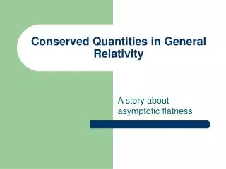
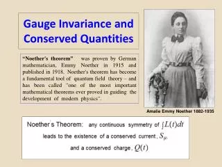
Gauge Invariance and Conserved Quantities “Noether's theorem” was proven by German mathematician, Emmy Noether in 1915 and published in 1918. Noether's theorem has become a fundamental tool of quantum field theory – and has been called "one of the most important mathematical theorems ever proved in guiding the development of modern physics". Amalie Emmy Noether 1882-1935
Consider the charged scalar field, and the following transformation on , where is a constant.
=1 Now suppose that can be varied continuously – so that we have an infinite number of small, continuous for which exp(i) = ’ and L L. The set of all these transformations, U = exp(i), form a group of operators. It is called U(1),a unitary group (because U*U = 1) Here the Hermitian conjugate is the complex conjugate because U is not a matrix.
Now, we have a more astounding result: we can vary the (complex) phase of the field operator, , everywhere in space by any continuous amount and not affect the “laws of physics” (that is the L) which govern the system! Note that everywhere in space the phase changes by the same . This is called a global symmetry. ’ Remember Emmy Noether!
With the help of Emmy Noether, we can prove that charge is conserved!
Deriving the conserved current and the conserved charge: Euler-Lagrange equation conserved current But our Lagrangian density also contains a *, so we obtain additional terms like the above, with replaced by *. In each case the Euler –Lagrange equations are satisfied. So, the remaining term is as follows:
The conserved current condition is To within an overall constant the conserved current is : a four – vector!
Now we need to evaluate . The great advantage of being a continuous constant is that there are an infinite number of very small which carry with them all the physics of the “continuity”. That is, with no loss of rigor we can assume is small!
Finally, the conserved current operator (to within an overall constant) for the charged, spin = 0, particle is Since we may adjust the overall constant to reflect the charge of the particle, we can replace with q. The formalism gives operator for charge, but not the numerical value.
The value of the charge is calculated from: integrate over time S0(t) incoming particle outgoing particle integrate over all space One obtains a number! p incoming outgoing
Next, we can do the integrations over d3x. Each gives a Dirac delta function in k and k’.
The time disappears! Q is time independent. The integration over k’ is done with the Dirac delta function from thed3x integration. The remaining integration over k will be done with the Dirac delta functions fromthe commutation relations. Note: + and/or – must be together.