Download
1 / 12
160 likes | 558 Vues
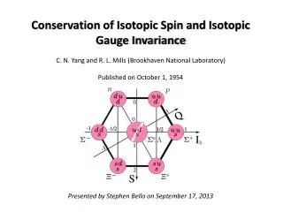
Conservation of Isotopic Spin and Isotopic Gauge Invariance C. N. Yang and R. L. Mills (Brookhaven National Laboratory) Published on October 1, 1954 Presented by Stephen Bello on September 17, 2013. So what exactly is Isospin /Isotopic Spin/Isobaric Spin?

E N D
Conservation of Isotopic Spin and Isotopic Gauge Invariance C. N. Yang and R. L. Mills (Brookhaven National Laboratory) Published on October 1, 1954 Presented by Stephen Bello on September 17, 2013
So what exactly is Isospin/Isotopic Spin/Isobaric Spin? • Theorized in 1932 by Werner Heisenberg to help explain symmetries between the proton and the newly discovered neutron. Two things existed that bolstered his argument: • The masses of the neutron and proton were nearly identical and are almost degenerate. Even though the proton had a positive charge and the neutron was neutral, they were almost the same in all other aspects. • The relative strength of the Strong Force (interaction) between the nucleons does not care whether it is n-p, p-p. or n-n. It acts as though both are the same type of particle. • Knowing all this, he came up with Isospin but it wasn’t until Eugene Wigner coined that phrase in 1937 that physicists referred to it as such. • Since protons and neutrons are baryons of spin ½, they were grouped together as nucleons due to their similar masses and interactions with other particles. It was easy to treat them as two states of the same particle. • Isospin would prove useful in the 1940’s when pions were discovered. The three flavors of pions (π+,π-,π0) could be given to an isospin triplet of +1,-1, or 0 and with the assumption isospin is conserved in nuclear interactions, pions could be easily added to the current nuclear theory.
What will be discussed A (brief) overview of the Isotopic Gauge Transformation and its Invariance Finding the Field Equations Quantizing the Field Equations for the b field Finding the Hamiltonians A discussion about the various properties of the quanta of the b field
The Isotopic Gauge Transformation • Let Ψ represent a wave function with two components that describes a field containing an isotopic spin ½. If there is an isotopic gauge transformation, Ψ is transformed as follows: Ψ = SΨ’ where S is a Unitary Matrix (2x2) with determinant unity. • It is required that any and all derivatives of Ψ to appear as: (dμ – iεBμ)Ψ. • Bμ = 2x2 matrices that are Hermitian for μ = 1,2,3 and anti-Hermitian for μ = 4. • The gauge invariance also requires that: S(dμ – iεBμ’)Ψ’ = (dμ – iεBμ)Ψ. • By combining these two equations we find the Isotopic Gauge Transformation on Bμ: • Bμ‘ = S-1BμS+(i/ε)S-1(dS/dxμ) • This last term is familiar to the gauge transformation of EM potentials • By defining Fμν = (dBμ/dxν)(dBν/dxμ) + iε(BμBν-BνBμ). • Combining this with the isotopic gauge transformation: Fμν‘ = S-1FμνS • The isotopic gauge transformation is valid for any S and the corresponding Bμ.
In the gauge transformation the matrix S-1(dS/dxμ) represents a linear combination of the isotopic spin angular momentum matrices Ti, where I = 1,2,3. In this format the B field is given by the form involving three-component vectors: • Bμ = 2bμT • The interaction between the field Ψ with isotopic spin with the b field can be found by a trivial replacement of the gradiant of Ψ with (dμ – 2iεbμT)Ψ.
The Field Equations • Finding the field equations for the b field involves only the isotopic gauge invariant quantities. Much like the EM case we can use the Lagrangian density: -¼ fμνfμν • Including a field with isotopic spin ½ does not make things overly complicated so we can use the total Lagrangian density to find the equations of motion: • We know that the divergence of Jμ doesn’t vanish so (dJμ/dxμ) = -2ebμxJμ. Something nice is that if we define ξμ = Jμ +2εbμ X fμν, substituting this into the equations of motion above lead to the equation of continuity: (dξμ /dxμ) = 0! • ξμ for μ = 1,2,3 are the isotopic spin current density while u = 4 is the isotopic spin density of the entire system.
By defining ξμ as a function of Jμ it’s shown that the isotopic spin of the system comes from both the spin-1/2 field (Jμ) as well as the bμ field. • The Hamiltonian derived from the total Lagrangian density can easily be shown to be positive definite in the absence of the field of isotopic spin-1/2. This is identical to what happens in electrodynamics. • We are not quite done. We still need to complete the equations of motion with the following condition: (dbμ/dxμ) = 0. This eliminates the scalar part of b and imposes a condition on the possible isotopic gauge transformations the system can undergo.
Now onto Quantization • Using the total Lagrangian density mentioned earlier makes quantizing really inconvenient. This is similar to what happens in electrodynamics and so we have to use a Lagrangian density that happens to not obviously be gauge invariant. • Using the equations of motion that comes from this Lagrangian, it can easily be implied that: If this is consistent with the supplementary equation we found earlier, if we put one space-like surface a = 0 together with da/dt =0, it follows that a = 0 at all times. Using this we can prove that the two Lagrangian densities mentioned so far are identical!
Finding the Hamiltonians • Using the canonical method of quantization with the gauge invariant Lagrangian density we can derive a Hamiltonian from it. This is virtually identical to the one found from the Field Equation Lagrangian, but only in respect to the supplementary condition. • Finding this Hamiltonian required defining the equation on the upper right. Doing this allowed us to obtain the equal-time commutation rule, whose relativistic invariance follows from Heisenberg and Pauli’s general proof for canonical methods of quantization. • These Hamilitonians will become useful later on.
Properties of the b Quanta • The quanta of the b field can clearly be seen to have spin unity and isotopic spin unity. The electric charge is also easily derived because every single interaction must satisfy the law of conservation of electric charge. Therefore the two states of the nucleon (which are again the neutron and proton) simply differ by charge unity. • Because they can transform or ‘evolve’ into each other through the emission/absorption of a single b quantum, there are three charge states: +e, -e, and 0. • By choosing the isotopic gauge so that the preferred direction is the z-axis in isotopic space, it can be found that for nucleons the electric charge is given by: Q = e(½ + ε-1Tz) and for the b quantum: Q = (e/ε)Tz. • We can easily fix the electric charge up to a additive constant for every single field that has isotopic spin: Q = e[Tz/ε + R] where R is equal and opposite for two charge conjugate fields.
So what is the mass of the b quantum? • It was argued that the Lagrangian would contain no quantity of the mass dimension if there was no nucleon field and then the mass of the b quantum would be zero. The only problem was that the b field, like every single field theory in existence, has divergences and therefore the dimensional arguments did not work. Primitive Divergences • If we apply F.J. Dyson’s approach to the b field we transform the interaction representation where the state vector Ψ has to satisfy i(dψ/dt) = HINTΨ. All of the matrix elements from the scattering matrix are formulated in terms of the Feynman diagram contributions. • In electrodynamics the electric charge conservation argues that the mass of the photon vanishes and arguments for this in the b field do not exist*. So at the time no conclusions about the b quantum mass could be determined.
Conclusions • Isospin was extremely useful as more and more particles were discovered. Many particles of similar mass but with varying units of charge would interact with the Strong Force nearly identically. As each new particle was found, they would be grouped into an isospinmultiplet that was based on the number of different charge states seen. • Two doublets of K mesons: I = -1/2 and -1/2 of (K-, K0)(K+, K0) • A single triplet I = 1 for Sigma baryons: (Σ+, Σ0, Σ-) • This multiplet structure put forth in Isotopic Spin would eventually be combined with the property of strangeness, leading to the creation of the Quark Model and modern Quantum Chromodynamics. • One can also apply isospins to quarks! More specifically the up and down quarks. The u and d quarks have similar masses but different charges (2/3e for up and -1/3e for down) and therefore will act identically under the Strong Force.