Introduction to computational plasma physics
Introduction to computational plasma physics. 雷奕安 62755208 , yalei@pku.edu.cn. 课程概况. http://www.phy.pku.edu.cn/~fusion/forum/viewtopic.php?t=77 上机 成绩评定为期末大作业. Related disciplines. Computation fluid dynamics (CFD) Applied mathematics, PDE, ODE Computational algorithms

Introduction to computational plasma physics
E N D
Presentation Transcript
Introduction to computational plasma physics 雷奕安 62755208,yalei@pku.edu.cn
课程概况 • http://www.phy.pku.edu.cn/~fusion/forum/viewtopic.php?t=77 • 上机 • 成绩评定为期末大作业
Related disciplines • Computation fluid dynamics (CFD) • Applied mathematics, PDE, ODE • Computational algorithms • Programming language, C, Fortran • Parallel programming, OpenMP, MPI • Plasma physics, space, fusion, … • Unix, Linux, …
Contents • What is plasma • Basic properties of plasma • Plasma simulation challenges • Simulation principles
What is plasma • Partially ionized gas, quasi-neutral • Widely existed • Fire, lightning, ionosphere, polar aurora • Stars, solar wind, interplanetary (stellar, galactic) medium, accretion disc, nebula • Lamps, neon signs, ozone generator, fusion energy, electric arc, laser-material interaction • Basic properties • Density, degree of ionization, temperature, conductivity, quasi-neutrality • magnetization
Basic properties • Temperature • Quasi-neutrality • Thermal speed • Plasma frequency • Plasma period
U→0 λD Debye length • System size and time • Debye shielding
Plasma parameter • Strong coupling • Weak coupling
Collision frequency • Mean-free-path • Collisional plasma • (Collisionless) • Collisioning frequency
Magnetized plasma • Anisotropic • Gyroradius • Gyrofrequency • Magnetization parameter • Plasma beta
Simulation challenges • Problem size: 1014 ~ 1024 particles • Debye sphere size: 102 ~ 106 particles • Time steps: 104 ~ 106 • Point particle, computational unstable, sigularities
Solution • No details, essence of the plasma • One or two dimension to reduce the size • No high frequency phenomenon, increase time step length • Reduce ND, mi / me • Smoothing particle charge, clouds • Fluidal approaches, single or double • Kinetic approaches, df/f
Simple Simulation • Electrostatic 1 dimensional simulation, ES1 • Self and applied electrostatic field • Applied magnetic field • Couple with both theory and experiment, and complementing them
Basic model • Field -> force -> motion -> field -> … • Field: Maxwell's equations • Force: Newton-Lorentz equations • Discretized time and space • Finite size particle • Beware of nonphysical effects
Equation of motion • vi, pi, trajectory • Integration method, fastest and least storage • Runge-Kutta • Leap-frog
Planet Problem x0 = 1; vx0 = 0; y0 = 0; vy0 = 1 read (*,*) dt N = 30/dt do i = 0, N+3 x1 = x0 + vx0*dt y1 = y0 + vy0*dt r = sqrt(x0*x0 + y0*y0) fx = -x0/r**3 fy = -y0/r**3 vx1 = vx0 + fx*dt vy1 = vy0 + fy*dt ! if(mod(i,N/10).eq.2) write(*,*) x0, y0, -1/r+(vx0*vx0+vy0*vy0)/2 x0 = x1; y0 = y1; vx0 = vx1; vy0 = vy1 enddo end Forward differencing
Planet Problem ./a.out > data 0.1 $ gnuplot Gnuplot> plot “data” u 1:2
Planet Problem ./a.out > data 0.01 $ gnuplot Gnuplot> plot “data” u 1:2
Planet Problem x0 = 1; vx0 = 0; y0 = 0; vy0 = 1 read (*,*) dt N = 30/dt x1 = x0 + vx0*dt y1 = y0 + vy0*dt xh0 = (x0+x1)/2; yh0 = (y0+y1)/2 do i = 0, N xh1 = xh0+vx0*dt; yh1 = yh0 + vy0*dt; r = sqrt(xh0*xh0 + yh0 *yh0 ) fx = -xh1/r**3 fy = -yh1/r**3 vx1 = vx0 + fx*dt vy1 = vy0 + fy*dt ! if(mod(i,N/100).eq.0) write(*,*) xh0, yh0, -1/r+(vx0*vx0+vy0*vy0)/2 xh0 = xh1; yh0 = yh1; vx0 = vx1; vy0 = vy1 enddo end Leap Frog
Planet Problem ./a.out > data 0.1 $ gnuplot Gnuplot> plot “data” u 1:2
Planet Problem ./a.out > data 0.01 $ gnuplot Gnuplot> plot “data” u 1:2
Field equations • Poisson’s equation
Field equations • Poisson’s equation is solvable • In periodic boundary conditions, fast Fourier transform (FFT) is used, filtering the high frequency part (smoothing), is easy to calculate
Particle and force weighting • Particle positions are continuous, but fields and charge density are not, interpolating • Zero-order weighting • First-order weighting, cloud-in-cell
Higher order weighting • Quadratic or cubic splines, rounds of roughness, reduces noise, more computation
Initial values • Number of particles and cells • Weighting method • Initial distribution and perturbation • The simplest case: perturbed cold plasma, with fixed ions. • Warm plasma, set velocities
Diagnostics • Graphical snapshots of the history • x, v, r, f, E, etc. • Not all ti • For particle quantities, phase space, velocity space, density in velocity • For grid quantities, charge density, potential, electrical field, electrostatic energy distribution in k space
Tests • Compare with theory and experiment, with answer known • Change nonphysical initial values (NP, NG, Dt, Dx, …) • Simple test problems
Server connection SshHost: 162.105.23.110, protocol: ssh2 Your username & password Vnc connectionIn ssh shell: “vncserver”, input vnc passwd, remember xwindow number Tightvnc: 162.105.23.110:xx (the xwindow number) Kill vncserver: “vncserver –kill :xx” (x-win no.)
Xes1 Xes1 document Xgrafix already compiled in /usr/local Xes1 makefile make ./xes1 -i inp/ee.inp LIBDIRS = -L/usr/local/lib -L/usr/lib -L/usr/X11R6/lib64
Clients Sshputty.exe Vncviewerhttp://www.phy.pku.edu.cn/~lei/vncviewer.exe Pscp: http://www.phy.pku.edu.cn/~lei/pscp.exe