Computational Plasma Physics
Computational Plasma Physics. Aims. To “cage” the cosmic medium: plasma. Get controle over its diversity. Get an overview of all the various Methods, Models, and Tools. Construct a modeling platform for the industry. Introduce young researchers/modellers. Has to be organized.

Computational Plasma Physics
E N D
Presentation Transcript
Computational Plasma Physics Aims To “cage” the cosmic medium: plasma Get controle over its diversity Get an overview of all the various Methods, Models, and Tools Construct a modeling platform for the industry Introduce young researchers/modellers
Has to be organized Structure of the course Lectures Joost van der Mullen (Tue) Wim Goedheer (FOM Nieuwegein) Annemie Bogaerts (Uni Antwerp) Ute Ebert (CWI) Practicum Bart Hartgers Wouter brok Bart Broks Examination: Projects
MathNum Interdiscipline SoftWArch Plasma Physics
Metal Halide Lamp Gravitation induced Segregation 10 mBar NaI and CeI3 in 10 bar Hg
The Philips QL lamp • Buffer argon (33 Pa) • Light Mercury (1 Pa) • Inductively coupled • Power 85 W Electrodeless lamp: long life time
350 sccm He 4 mm i.d. 60 mm transformer CCP Spectrochemical Plasma Sources 18 mm i.d. central channel (CC) induction coil active zone (AZ) 15l/min outer flow intermediate flow central flow ICP Open air • 10- 50 W • 0.3 - 2 kW • 100 kHz; • 100 MHz • Helium • Argon
Microwave Plasma Torch (MPT) Frequency 2.45 GHz Power 100W Argon flushing into The open air
Booming Plasma Technology Interest increasing rapidly Material sciences (sputter) deposition CD, IC, DVD, nanotubes, solar-cells, Environmental gas-cleaning, ozon production, waste destruction Light Lamps, Lasers, Displays: Visible + EUV Propulsion Laser Wake field, Thrusters Etc. Etc
Continuum or Particle And/Or ?? “Hybrid” Components Material Particles Neutral Charged Dust Fields Photons Note the various interactions
Particles, Momentum, Energy Plasma ChemistryVolumeParticles Surface Particles + environment Plasma PropulsionMomentum Plasma LightEnergy
Ordering Particles Chemistry m Momentum Propulsion mv Energy Conversion 1/2mv2
Energy Coupling; Ordering in frequency DC Cascaded Arcs Deposition/Lightsources Pulsed DC pHollowCathodeD EUV gen/switches Corona Disch. Volume cleaning AC HID/FL lamps Welding/Cutting/light CC GEC cell etc. Etching/Depo/ SpectrChem IC QL lamp Licht/ Spectrochemistry Wave Surfatron Material processing Laser ProPl Ablation Cutting/ EUV generation
Momentum Via E field: Plasma Propulsion Sheath: ion acceleration Ohms law: electon current Via p : expansion Cascaded Arc
Atomic Molecular Low High pressure Chemistry; global ordering
electrons, M-ions A-ions atoms, molecules; Radicals etc. Final Chemistry Chemistry; finer ordering Plasma gas i.e. Hg in a FLamp Buffergas i.e. Hg in a HID lamp; Ar in a FL Reduction diffusion Enhencing resistance Starting gas Xe in HID lamp
Hybride Quasi Free Flight mean free paths large mfp > L Sampling and tracking Transport Modes Fluid mean free paths small mfp << L There are many conditions for which some plasma components behave “fluid-like” whereas others are more “particle-like” Hybride models have large application fields
Particles Plasma Particles Energy Energy Momentum Momentum Particles: Plasma Chemistry Energy: Plasma Light Momentum: Plasma Propulsion
Fluid models; a flavor Continuum approach: Differentiation/Integration possible Not jumping over neighbour’s garden
Source Discretizing a Fluid: Control Volumes Plasma Particles Particles Energy Energy Momentum Momentum For any transportable quantity Transport via boundaries
How many species? How many species? Examples of transportables Densities Momenta in three directions Mean energy (temperature) of electrons Mean energy (temperature) of heavies As we will see: in many cases energy: 2T momentum: Drift Diffusion Species depending on equilibrium departure
Mean properties Nodal Points Transport at boundaries = Source, t + = S Steady State Transient General structure: = u -D Convection Diffusion Nodal Point communicating via Boundaries Transport Fluxes: Linking CV (or NP’s) -
Other Example: Poisson: .E = /o = S = u -D E = -V Thus no “convection” Modularity Thus: The Fluid Eqns: Balance of Particles Momentum Energy The Momenta of the Boltzmann Transport Eqn. Treated all as -equation
The Variety D S Temperature Heat cond Heat gen Momentum Viscosity Force Density Diffusion Creation Molecules atoms ions/electrons etc.
Source of ions 1 Sink in Energy 2 Coupling different -equations Associated with
Advantages of the -approach The same solution procedure: the same base class Possible to combine all the s in one big Matrix-vector eqn.
T Continuum t + = S Tin Rod Tout x 0 + T = 0 Take k = Cst MathNumerics: a FlavorSourceless-Diffusion T = Cst T = - kT -T /k =T
Continuum Tin Rod Tout Discretized Intuition; T = Cst T2 = (T1 + T3)/2 1 2 3 4 Tin -2T1 + T2= 0 T1 - 2T2 + T3 = 0 T2 - 2T3 + T4 = 0 T3 - 2T4 + Tout = 0 2T2 = T1 + T3 Discretized
In matrix: M T = b A Sparce Matrix Many zeros Matrix Representation 1 2 3 4 -Tin 0 0 -Tout T1 T2 T3 T4 1 2 3 4 - 2 1 1 -2 1 1 -2 1 1 -2 =
Sourceless-Diffusion in two dimensions 1 1 – 4 1 1 N W P E S T5 = (T2 + T4 +T6 + T8 ) /4 Provided k = Cst !! In general:
If k Cst Convection Diffusion More general S-less Diffusion/Convection
Source of ions Example ions: nu+ = P+ - n+D+ Recombination Ordering the Sources = S S = P - L L ~ D Source combination Production and Loss Large local - value in general leads to large Loss
The number of -equations How many -equations do we need ?? The number of transportables Depends on the degree of equilibrium departure Method of disturbed Bilateral Relations dBR Insight in equilibrium departure global model ne, Te and Th
Particles Plasma Particles Energy Energy Momentum Momentum
Plasma Artist Impression Input and Output Intermediated by Vivid Internal Activity
Internal Activity Global Structure Inlet Outlet The In/Efflux couple will disturb internal Equilibrium Inlet side will be pushed up; Outlet pushed down But when do we have equilibrium ???
N f N b TE: Collection of Bilateral Relations TE Equilibrium in (violet) thermal dynamics DB Equilibrium on each level (each ) for any process-couple along the same route
t = Nt Disturbance of BR by an Efflux N f N b Equilibrium Condition: t/b << 1 or t b << 1 The escape per balance time must be small
y = N/Neq Non-Equilibrium N f = N b + N t y() = y()[1+ (tb)] Equilibrium Departure N f N b Equilibrium N eqf = N eqb
The Nature of the Processes; PROPER Balances =1 =+ Emission = Absorption Planck Excitation = Deexcitation Boltzmann Ionization = Recombin Saha Kinetic Energy Exchange Maxwell
Equilibrium Any situation aspects Non-Equilibrium Saha Boltzmann Planck Maxwell pLSE pLBE pLPE pLME Nature Nomenclature induced by dBR TE, LTE, pLTE ?? Partial Equilibrium Proper Balances
Forward and corr. Backward Proper MR and Energy Conservation give standard relations Backward negligible Improper Assumption: d/dt = 0 Analytical expressions (!?) Proper versus Improper balances
=2 =1 Example pLPE Intense laser irradiates transition: Proper balance Absorption St.Emission h= E Look for comparable TE situation T : exp-E/kT=1 (1) = (2) • (p) = n(p)/g(p) number density of a state; n(p) = number density of atoms in level p g(p) = number of states in level p
Ion state Ground state Ionization flow Influx Outflux Approaching continuum: Equi. restoration rates increase Look for comparable TE situation Saha equation ruled by electrons from continuum Example pLSE s(p) = (ne/2) (n+/g+) [h3/(2mekTe)3/2] exp (Ip/kTe)
s(p) = e + [V(Te) ] exp (Ip/kTe) That is Look at balance Ap A+ + e A+ + e bound free pair The Saha density: mnemonic s(p) = (ne/2) (n+/g+) [h3/(2mekTe)3/2] exp (Ip/kTe) Number density of bound {e +} pairs in state p: s(p) Equals the density of pairs within V(Te) e + [V(Te) ] Weighted with the Boltzmann factor exp (Ip/kTe)
Escape of Photons Restoring: Proper Boltzmann Tends to b(2) = b(1) exp { -E12/kTe} The Corona Balance: an improper balance a b y() = y()[1+ (tb)B] with (tb)B=A/ne K(2,1) The larger ne the smaller departure
p =1 =2 N (p)p-9 General: Impact Radiation Leak y(p) = y(1)[1+ tb]-1 with tb =A*(p)/ne K(p,1) Define: N= A(p)/neK(p) A(p) p-4.5 K(p) p4
Ion state Ground state Ionization flow Influx Outflux b = n/ns pLSE settles for Ip 0 since (t/b)S 0 Ion Efflux Effecting the ASDF
b=+ a=1 t = n+t = .n+w+ n+w+ = -Da.n Diffusion For single ionized ns(1)~ nen+= ne2 If Ambipolar Diffusion Dominates t = Da/L2 b(1) = (tb)s= t/ (ns(1) Sion) Cb (A) x 108 Da (neL)-2 Moderate deviations for large ne, large L and small Da
Ion Efflux Effecting the EEDF F(E) = bulk = tail E E12