Analysis and Interpretation: Analysis of Variance (ANOVA)
370 likes | 847 Vues
Analysis and Interpretation: Analysis of Variance (ANOVA). Chris Fowler. Contents & Outcomes. Four Basic Questions: Why use ANOVA? Multiple comparisons of means More Complex Designs Main effects and interactions What is ANOVA? Why analyse variance? How do we interpret the results?

Analysis and Interpretation: Analysis of Variance (ANOVA)
E N D
Presentation Transcript
Analysis and Interpretation:Analysis of Variance (ANOVA) Chris Fowler
Contents & Outcomes Four Basic Questions: • Why use ANOVA? • Multiple comparisons of means • More Complex Designs • Main effects and interactions • What is ANOVA? • Why analyse variance? • How do we interpret the results? • Summary and Mean Tables • Statistical v’s theoretical significance • When to use it? • Assumptions (Parameters)
Scope • The presentation will not focus on: • statistical theory (beyond what is necessary) • computations and formulae (use a computer!) • But it will focus on: • making sense of the results • helping you to choose the right design • However in ANOVA the design, data collection, and analysis become inseparable
1. Why use ANOVA? • Multiple (more than 2) simultaneous comparisons of means. • Comparison of 3 means using a T test would mean undertaking 3 analysis A vs B A vs C B vs C • 4 comparisons = 6 tests; or N(N-1) 2 Where N=Number of Means being compared • ANOVA allows the simultaneous comparison of the means – only one test • So what’s the problem? • Type 1 errors • Loss of information (interactions)
Making a Type 1 error • A significance level tells you the probability of rejecting the Null Hypothesis when it is in fact true. • P<0.05 means that there is less than 5 out 100 chance of incorrectly rejecting the Null hypothesis. Or there is a 5% chance of making an error called a type 1 error. • So your significance level states the probability of making a Type 1 error • Every additional comparison you make increase the chances of a type 1 error (so if you do 100 comparisons – 5 are likely to be false – but which five?).
Type I and Type II Errors Note that 1-beta equals the power of a test
But….. • A significant main effect means that overall there is a significant difference between means . • But one mean may not be significantly different from one of the others. • To make specific comparisons you can do a ‘Planned or Unplanned Comparison’. • Equally you can test for linear or nonlinear trends (Trend tests). • Both use weighted coefficients that must sum to zero and total number of comparison/trends cannot exceed the total number of DF (L-1) for the effect you are examining. (You are partitioning the variance).
Example Coefficients for Planned Comparisons • Four Levels (L1,L2,L3 and L4) L1 L2 L3 L4 +3 vs -1 and -1 and -1 +1 vs -1 0 0 +1 and +1 vs -1 and -1 Remember they are planned – you were expecting to find a difference. There are unplanned comparisons for more explorative analysis but be aware of post hoc analysis.
Exercise • Use the coefficients and draw the trends on a graph.
More Complex Designs • A Simple design (or one way ANOVA) only has a single independent variable (Factor) with three or more levels. For example The effects of Noise on memory retention. Three levels of Noise (High, Medium and Low) and each subjects’ score is the number of words remembered (out of 20) This would be One way Between subject factorial design. The within S equivalent would have each subject undertaking all the Noise conditions.
Two Way ANOVA • You have two independent variables (Factors). • For example as well as noise you have Task Difficulty (Easy & Hard) as a variable. Easy Hard H M L H M L X X X X X X X X X X X X A within-S example as above but S1 X X X X X X S2 X X X X X X
Within AND Between Subject Designs (Mixed or Split plot) Where one Factor is B-S and the other is W-S Eg H M L Easy S1 X X X S2 X X X Hard S6 X X X S7 X X X
Main Effects and Interactions • More Complex designs (more than One way) allow you not only to explore the main effects of the individual variables but also the interaction between the variables. • These can be two way (A x B), three way (AxBxC) , four ways and so on. • A two way ANOVA (A,B) only has one interaction (AxB); a three way has three interactions (AxB; AxC and AxBxC) and so on.
2. What is ANOVA? • How can analysing variance tells us about differences between means?
Analysing the Variance Sample 1 and 2 are very similar and combining them makes little difference to the overall mean (10.5) or Variance (9.17) But Sample 3 has a much lower mean, and although it starts with same variance as the other two, if you combine it with sample 1 and 2 the variance will increase (15.95) They all started with same variance so the increase in variance can only be attributed to difference between the means.
But….. • This only works if you assume homogeneity of variance. • ANOVA is based on statistical theory relating to populations rather than samples, but under certain conditions we can assume that the sample is unbiased estimate of our population hence inferring from samples about populations • The conditions are stated in the central limit theorem (mean, variance and shape).
And…. • Any treatment effect also contains sampling error so we need to calculate the error separately. The greater the treatment effect the greater disparity between the two. • If there is no treatment effect (all error) then dividing the treatment effect by error (a residual) will result in a ratio of 1 (the F ratio)* • The greater the treatment effect the greater the value of F. • To decide whether the F-ratio is significant (ie you can reject the null hypothesis) you need to look up in a table the probability of getter that particular F value for that particular F distribution. • The particular distribution is determined by number of degrees of freedom associated with your treatment and error effects * In a perfect world you would never get an F value less than one, but because we use estimates an F<1 can occur.
3. Interpreting the results • Have the tables of means and ANOVA summary table at hand • Select and interpret those means for which you have predicted effects on the basis of your hypotheses. • Interpret any significant but unpredicted effects (with caution) but use a ‘two-tail’ test (halves the probability) or increase the significance level (P<0.01 rather than P<0.05)
ANOVA Summary Table Simple Two-way ANOVA:
An Example Hypothesis – Background noise has a masking effect that helps students concentrate better, particularly on difficult tasks Independent Variables: • Three levels of background noise’ (65db, 75db & 85dbs) • Two levels of task difficulty (easy and hard) Dependent Variable • Number of key points recalled from a piece of text.
Raw Data Equal Cell sizes (n=5) A 2 x 3 Factorial BS Design
Interaction x 8 6 o x 4 o x Easy x 2 o o Hard x o 85 65 75
Results • That more items were recalled from the easy (4.6) compared to the hard task (3.6) (F=32.93, df 1, 24, P<0.001). This was expected. • That as noise increases, recall improves (F=99.31, df 2, 24, P<0.001). • That the effect of the noise diminishes as the tasks becomes harder (F=8.96, df 2, 24, P<0.05) or the more difficult the task the less background noise should be used.
Theoretical vs Statistical Significance • Be wary of: • Post hoc explanation (changing your hypothesis after analysing your data) • Data Trawling (capturing as much data as you can rather than the data you need) • Post mortem data analysis (keep on analysing in unintended ways until you find something significant) • Data checking (only checking your results when you have no significant findings) • Data exclusion (getting rid of those awkward scores!)
And…. • Something that is statistically significant may have no or limited theoretical significance • Equally something that is statistically non significant may have theoretical significance (pressure to publish only significant results).
4. When to use ANOVA • ANOVA is a very powerful test , but its use is based on certain assumptions: • The population distribution from which the sample was drawn from should be normally distributed. • The observations should be independent (usually assured through random sampling and assignment) • Measurements should be made on an interval or ratio scale (but ordinal data can be transformed into normal scores). • There should be homogeneity of variance (usually OK if equal sample sizes are used).
But…. • ANOVA is a very robust test and can sustain breaches in its assumptions. • However, if you think some of the assumptions are breached and a equivalent non-parametric test is available then you should use the non parametric version.