Software Project Planning
Software Project Planning. Software Project Planning. After the finalisation of SRS, we would like to estimate size, cost and development time of the project. Also, in many cases, customer may like to know the cost and development time even prior to finalisation of the SRS.


Software Project Planning
E N D
Presentation Transcript
Software Project Planning
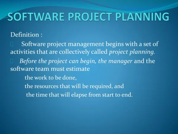
Software Project Planning After the finalisation of SRS, we would like to estimate size, cost and development time of the project. Also, in many cases, customer may like to know the cost and development time even prior to finalisation of the SRS.
Software Project Planning In order to conduct a successful software project, we must understand: • Scope of work to be done • The risk to be incurred • The resources required • The task to be accomplished • The cost to be expended • The schedule to be followed
Size estimation Cost estimation Development time Resources requirements Project scheduling Software Project Planning Software planning begins before technical work starts, continues as the software evolves from concept to reality, and culminates only when the software is retired. The various steps of planning activities are illustrated shown below :
Software Project Planning Size Estimation Lines of Code (LOC) If LOC is simply a count of the number of lines then figure shown below contains 18 LOC . When comments and blank lines are ignored, the program in figure shown below contains 17 LOC.
Software Project Planning Growth of Lines of Code (LOC)
Software Project Planning Furthermore, if the main interest is the size of the program for specific functionality, it may be reasonable to include executable statements. The only executable statements in figure shown above are in lines 5-17 leading to a count of 13. The differences in the counts are 18 to 17 to 13. One can easily see the potential for major discrepancies for large programs with many comments or programs written in language that allow a large number of descriptive but non-executable statement. Conte has defined lines of code as:
Software Project Planning “A line of code is any line of program text that is not a comment or blank line, regardless of the number of statements or fragments of statements on the line. This specifically includes all lines containing program header, declaration, and executable and non-executable statements”. This is the predominant definition for lines of code used by researchers. By this definition, figure shown above has 17 LOC.
Software Project Planning Function Count Alan Albrecht while working for IBM, recognized the problem in size measurement in the 1970s, and developed a technique (which he called Function Point Analysis), which appeared to be a solution to the size measurement problem.
Software Project Planning The principle of Albrecht’s function point analysis (FPA) is that a system is decomposed into functional units. • Inputs : information entering the system • Outputs : information leaving the system • Enquiries : requests for instant access to information • Internal logical files : information held within the system • External interface files : information held by other system that is used by the system being analyzed.
User Inquiries Other applications ILF Inputs EIF User Outputs ILF: Internal logical files EIF: External interfaces System Software Project Planning The FPA functional units are shown in figure given below: FPAs functional units System
Software Project Planning The five functional units are divided in two categories: (i) Data function types • Internal Logical Files (ILF): A user identifiable group of logical related data or control information maintained within the system. • External Interface files (EIF): A user identifiable group of logically related data or control information referenced by the system, but maintained within another system. This means that EIF counted for one system, may be an ILF in another system.
Software Project Planning (ii) Transactional function types • External Input (EI): An EI processes data or control information that comes from outside the system. The EI is an elementary process, which is the smallest unit of activity that is meaningful to the end user in the business. • External Output (EO): An EO is an elementary process that generate data or control information to be sent out side the system. • External Inquiry (EQ): An EQ is an elementary process that is made up to an input output combination that result in data retrieval.
Software Project Planning Special features • Function point approach is independent of the language, tools, or methodologies used for implementation; i.e. they do not take into consideration programming languages, data base management systems, processing hardware or any other data base technology. • Function points can be estimated from requirement specification or design specification, thus making it possible to estimate development efforts in early phases of development.
Software Project Planning • Function points are directly linked to the statement of requirements; any change of requirements can easily be followed by a re-estimate. • Function points are based on the system user’s external view of the system, non-technical users of the software system have a better understanding of what function points are measuring.
Software Project Planning Counting function points Table 1 : Functional units with weighting factors
Software Project Planning Table 2: UFP calculation table Functional Unit Totals Functional Units Complexity Totals Count Complexity External Inputs (EIs) = Low x 3 Average x 4 = High x 6 = External Outputs (EOs) = Low x 4 Average x 5 = High x 7 = External Inquiries (EQs) = Low x 3 Average x 4 = High x 6 = External logical Files (ILFs) = Low x 7 Average x 10 = High x 15 = External Interface Files (EIFs) = Low x 5 Average x 7 = High x 10 = Total Unadjusted Function Point Count
Software Project Planning The weighting factors are identified for all functional units and multiplied with the functional units accordingly. The procedure for the calculation of Unadjusted Function Point (UFP) is given in table shown above.
Software Project Planning The procedure for the calculation of UFP in mathematical form is given below: Where i indicate the row and j indicates the column of Table 1 Wij : It is the entry of the ith row and jth column of the table 1 Zij : It is the count of the number of functional units of Type i that have been classified as having the complexity corresponding to column j.
Software Project Planning Organisations that use function point methods develop a criterion for determining whether a particular entry is Low, Average or High. Nonetheless, the determination of complexity is somewhat subjective. FP = UFP * CAF Where CAF is complexity adjustment factor and is equal to [0.65 + 0.01 x ΣF]. The Fi (i=1 to 14) are the degree of influence and are based on responses to questions noted in table 3.
Software Project Planning Table 3 : Computing function points. 1 Rate each factor on a scale of 0 to 5. 0 1 2 3 5 4 Average Essential Significant No Influence Incidental Moderate Number of factors considered ( Fi ) 1. Does the system require reliable backup and recovery ? 2. Is data communication required ? 3. Are there distributed processing functions ? 4. Is performance critical ? 5. Will the system run in an existing heavily utilized operational environment ? 6. Does the system require on line data entry ? 7. Does the on line data entry require the input transaction to be built over multiple screens or operations ? 8. Are the master files updated on line ? 9. Is the inputs, outputs, files, or inquiries complex ? 10. Is the internal processing complex ? 11. Is the code designed to be reusable ? 12. Are conversion and installation included in the design ? 13. Is the system designed for multiple installation in different organizations ? 14. Is the application designed to facilitate change and ease of use by the user ?
Software Project Planning Functions points may compute the following important metrics: Productivity = FP / persons-months Quality = Defects / FP Cost = Rupees / FP Documentation = Pages of documentation per FP These metrics are controversial and are not universally acceptable. There are standards issued by the International Functions Point User Group [IFPUG, covering the Albrecht method) and the United Kingdom Function Point User Group (UFPGU, covering the MK11 method). An ISO standard for function point method is also being developed.
Software Project Planning Example: 1 Consider a project with the following functional units: Number of user inputs = 50 Number of user outputs = 40 Number of user enquiries = 35 Number of user files = 06 Number of external interfaces = 04 Assume all complexity adjustment factors and weighting factors are average. Compute the function points for the project.
Software Project Planning Solution We know UFP = 50 x 4 + 40 x 5 + 35 x 4 + 6 x 10 + 4 x 7 = 200 + 200 + 140 + 60 + 28 = 628 CAF = (0.65 + 0.01 ΣFi) = (0.65 + 0.01 (14 x 3)) = 0.65 + 0.42 = 1.07 FP = UFP x CAF = 628 x 1.07 = 672
Software Project Planning Example: 2 An application has the following: 10 low external inputs, 12 high external outputs, 20 low internal logical files, 15 high external interface files, 12 average external inquiries, and a value of complexity adjustment factor of 1.10. What are the unadjusted and adjusted function point counts ?
Software Project Planning Solution Unadjusted function point counts may be calculated using as: = 10 x 3 + 12 x 7 + 20 x 7 + 15 + 10 + 12 x 4 = 30 + 84 +140 + 150 + 48 = 452 FP = UFP x CAF = 452 x 1.10 = 497.2.
Software Project Planning • Example: 3 • Consider a project with the following parameters. • (i) External Inputs: • 10 with low complexity • 15 with average complexity • 17 with high complexity • (ii) External Outputs: • 6 with low complexity • 13 with high complexity • (iii) External Inquiries: • (a) 3 with low complexity • (b) 4 with average complexity • (c) 2 high complexity
Software Project Planning • (iv) Internal logical files: • 2 with average complexity • 1 with high complexity • (v) External Interface files: • 9 with low complexity • In addition to above, system requires • Significant data communication • Performance is very critical • Designed code may be moderately reusable • System is not designed for multiple installation in different organizations. Other complexity adjustment factors are treated as average. Compute the function points for the project.
Software Project Planning Solution: Unadjusted function points may be counted using table 2 Functional Unit Totals Functional Units Complexity Totals Count Complexity External Inputs (EIs) = 10 Low x 3 30 Average x 4 = 15 60 High x 6 = 192 17 102 External Outputs (EOs) 6 24 = Low x 4 Average x 5 0 = 0 High x 7 115 13 = 91 External Inquiries (EQs) 3 9 = Low x 3 Average x 4 4 = 16 High x 6 37 2 = 12 External logical Files (ILFs) 0 = 0 Low x 7 Average x 10 = 2 20 High x 15 = 35 1 15 External Interface Files (EIFs) 9 45 = Low x 5 Average x 7 0 = 0 High x 10 45 0 = 0 424 Total Unadjusted Function Point Count
Software Project Planning 3+4+3+5+3+3+3+3+3+3+2+3+0+3=41 CAF = (0.65 + 0.01 x ΣFi) = (0.65 + 0.01 x 41) = 1.06 FP = UFP x CAF = 424 x 1.06 = 449.44 Hence FP = 449
Software Project Planning Relative Cost of Software Phases
Software Project Planning Cost to Detect and Fix Faults Relative Cost to detect and correct fault
Software Project Planning Cost Estimation A number of estimation techniques have been developed and are having following attributes in common : • Project scope must be established in advanced • Software metrics are used as a basic from which estimates are made • The project is broken into small pieces which are estimated individually To achieve reliable cost and schedule estimates, a number of options arise: • Delay estimation until late in project • Use simple decomposition techniques to generate project cost and schedule estimates • Develop empirical models for estimation
Software Project Planning MODELS Static, Single Variable Models Static, Single Multivariable Models
Software Project Planning Static, Single Variable Models Methods using this model use an equation to estimate the desired values such as cost, time, effort, etc. They all depend on the same variable used as predictor (say, size). An example of the most common equations is : (i) C = a Lb E = 1.4 L0.93 DOC = 30.4 L0.90 D = 4.6 L0.26 Effort (E in Person-months), documentation (DOC, in number of pages) and duration (D, in months) are calculated from the number of lines of code (L, in thousands of lines) used as a predictor.
Software Project Planning Static, Multivariable Models These models are often based on equation (i), they actually depend on several variables representing various aspects of the software development environment, for example method used, user participation, customer oriented changes, memory constraints, etc. E = 5.2 L0.91 D = 4.1 L0.36 The productivity index uses 29 variables which are found to be highly correlated to productivity as follows:
Software Project Planning Example: 4 Compare the Walston-Felix model with the SEL model on a software development expected to involve 8 person-years of effort. • Calculate the number of lines of source code that can be produced. • Calculate the duration of the development. • Calculate the productivity in LOC/PY • Calculate the average manning
Software Project Planning Solution The amount of manpower involved = 8 PY = 96 person-months (a) Number of lines of source code can be obtained by reversing equation to give: L = (E/a)1/b Then L(SEL) = (96/1.4)1/0.93 = 94264 LOC L(SEL) = (96/5.2)1/0.91 = 24632 LOC.
Software Project Planning (b) Duration in months can be calculated by means of equation D(SEL) = 4.6 (94.264)0.26 = 4.6 (94.264)0.26 = 15 months D(W-F) = 4.1 L0.36 = 4.1(24.632)0.36 = 13 months (c) Productivity is the lines of code produced per person/month (year)
Software Project Planning (d) Average manning is the average number of persons required per month in the project.
Software Project Planning The Constructive Cost Model (COCOMO) Constructive Cost model (COCOMO) Intermediate Detailed Basic Model proposed by B. W. Boehm’s through his book Software Engineering Economics in 1981
Software Project Planning COCOMO applied to Semidetached model Organic model Embedded model
Software Project Planning Familiar & In house Small size project, experienced developers in the familiar environment. For example, pay roll, inventory projects etc. Organic Typically 2-50 KLOC Little Not tight Medium Medium Medium Medium size project, Medium size team, Average previous experience on similar project. For example: Utility systems like compilers, database systems, editors etc. Semi detached Typically 50-300 KLOC Complex Hardware/ customer Interfaces required Significant Tight Typically over 300 KLOC Large project, Real time systems, Complex interfaces, Very little previous experience. For example: ATMs, Air Traffic Control etc. Embedded Table 4:The comparison of three COCOMO modes
Software Project Planning Basic Model Basic COCOMO model takes the form where E is effort applied in Person-Months, and D is the development time in months. The coefficients ab, bb, cb and db are given in table 4 (a).
Software Project ab bb cb db Organic 2.4 1.05 2.5 0.38 Semidetached 3.0 1.12 2.5 0.35 Embedded 3.6 1.20 2.5 0.32 Software Project Planning Table 4(a):Basic COCOMO coefficients
Software Project Planning When effort and development time are known, the average staff size to complete the project may be calculated as: Average staff size When project size is known, the productivity level may be calculated as: Productivity
Software Project Planning Example: 5 Suppose that a project was estimated to be 400 KLOC. Calculate the effort and development time for each of the three modes i.e., organic, semidetached and embedded.
Software Project Planning Solution The basic COCOMO equation take the form: Estimated size of the project = 400 KLOC (i) Organic mode E = 2.4(400)1.5 = 1295.31 PM D = 2.5(1295.31)0.38 = 38.07 PM
Software Project Planning (ii) Semidetached mode E = 3.0(400)1.12 = 2462.79 PM D = 2.5(2462.79)0.35 = 38.45 PM (iii) Embedded mode E = 3.6(400)1.20 = 4772.81 PM D = 2.5(4772.8)0.32 = 38 PM
Software Project Planning Example: 6 A project size of 200 KLOC is to be developed. Software development team has average experience on similar type of projects. The project schedule is not very tight. Calculate the effort, development time, average staff size and productivity of the project.