Download
1 / 7
90 likes | 741 Vues
Lectures 24-25 Electronic structure of Coordination Compounds 1) Crystal Field Theory. Considers only electrostatic interactions between the ligands and the metal ion. Ligands are considered as point charges creating an electrostatic field of a particular symmetry.

E N D
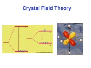
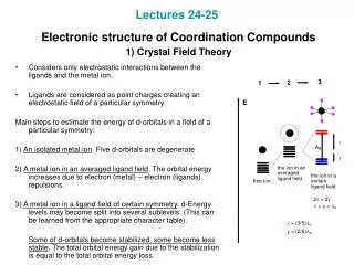
Lectures 24-25 Electronic structure of Coordination Compounds 1) Crystal Field Theory • Considers only electrostatic interactions between the ligands and the metal ion. • Ligands are considered as point charges creating an electrostatic field of a particular symmetry. Main steps to estimate the energy of d-orbitals in a field of a particular symmetry: 1) An isolated metal ion. Five d-orbitals are degenerate 2) A metal ion in an averaged ligand field. The orbital energy increases due to electron (metal) – electron (ligands) repulsions. 3) A metal ion in a ligand field of certain symmetry. d-Energy levels may become split into several sublevels. (This can be learned from the appropriate character table). Some of d-orbitals become stabilized, some become less stable. The total orbital energy gain due to the stabilization is equal to the total orbital energy loss.
2) Octahedral field. ML6 complexes • In the field of Oh symmetry five degenerate d-orbitals will be split into two sets, t2g and eg orbitals (check the Oh point group character table) • Three t2g orbitals be stabilized by 0.4Do and two eg orbitals will be destabilized by 0.6Do
3) Some consequences of d-orbital splitting • Magnetism. In the case of large Do we observe low-spin, while for small Dohigh-spin complexes (d4-d7 configurations). • Energy. If the occupancy (x) of the orbitals stabilized by a ligand field is more than that of the destabilized orbitals (y), the complex becomes more stable by CFSE which is (0.4x-0.6y)Do for octahedral species. • For d0, d5 (high-spin) and d10 complexes CFSE is always zero. • Redox potentials. Some oxidation states may become more stable when stabilized orbitals are fully occupied. So, d6 configuration becomes more stable than d7 as Do increases. CoL62+ = CoL63+ + e- E0= -1.8 (L=H2O) … +0.8 V (L=CN-) • M-L bond lengths and Ionic radii of Mn+ are smaller for low-spin complexes and have a minimum for d6 configuration (low spin). R, Å, of M3+: 0.87 (Sc), 0.81 (Ti), 0.78 (V), 0.74 (Cr), 0.72 (Mn), 0.69 (Fe), 0.67 (Co), 0.71 (Ni), … 0.78 (Ga)
4) Magnetism of octahedral transition metal complexes • The number of unpaired electrons n in a metal complex can be derived from the experimentally determined magnetic susceptibility cM. • cM is related to magnetic moment m≈2.84(cMT)1/2 (Bohr magnetons) • mis related to n: m≈ [n(n+2)]1/2. • Calculated magnetic moments for octahedral 3d metal complexes, ML6:
5) d-Orbital splitting in the fields of various symmetries • The d-orbital splittings presented on diagram correspond to the cases of cubic shape MX8 (Oh), tetrahedral shape MX4 (Td), icosahedral shape MX12 (Ih), octahedral shape MX6 (Oh) and square planar shape MX4 (D4h).
6) High and low spin complexes of various geometries • d-d Electron-electron repulsions in d4-d7 metal complexes (3d) correspond to the energy of 14000-25000 cm-1. If D > 14000-25000cm-1, the complex is low spin. • For octahedral complexes Do ranges from 9000 to 45000 cm-1. It is therefore common to observe both high and low spin octahedral species. • For tetrahedral complexes Dt = (4/9)Do ranges from 4000 to 16000 cm-1. Low spin tetrahedral complexes are very rare. • For square planar complexes D is very large. Even with weak field ligands high-spin d8 complexes are unknown (but known for d6). • Sometimes complexes of different configuration and magnetic properties coexist in equilibrium in solution. For the Ni(II) complexes shown below m=0bM (R = Me; square planar); 3.3 (R = tBu; tetrahedral) and 0-3.3 (R = iPr; both)
7) Factors affecting the magnitude of D • Higher oxidation states of the metal atom correspond to larger D : D=10,200 cm-1 for [CoII(NH3)6]2+ and 22,870 cm-1 for [CoIII(NH3)6]3+ D=32,200 cm-1 for [FeII(CN)6]4- and 35,000 cm-1 for [FeIII(CN)6]3- • In groups heavier analogues have larger D. For hexaammine complexes [MIII(NH3)6]3+:D = 22,870 cm-1 (Co) 34,100 cm-1 (Rh) 41,200 cm-1 (Ir) • Geometry of the metal coordination unit affects D greatly. For example, tetrahedral complexes ML4 have smaller D than octahedral ones ML6: D = 10,200 cm-1 for [CoII(NH3)6]2+ 5,900 cm-1 for [CoII(NH3)4]2+ • Ligands can be arranged in a spectrochemicalseries according to their ability to increase D at a given metal center: I- < Br- < Cl- < F- , OH- < H2O < NH3 < NO2- < Me- < CN- < CO For [CoIIIL6] we have D, cm-1: 13,100 (F), 20,760 (H2O), 22,870 (NH3) For [CrIIIL6] we have D, cm-1: 15,060 (F), 17,400 (H2O),26,600 (CN)