Download
1 / 55
560 likes | 610 Vues
Learn about logical clocks, Lamport's algorithm, happened-before relation, and creating a total order of events in distributed systems. Understand how to synchronize events across different processes accurately.

E N D
Topics • Logical clocks • Totally-Ordered Multicasting • Vector timestamps
Readings • Van Steen and Tanenbaum: 5.2 • Coulouris: 10.4 • L. Lamport, “Time, Clocks and the Ordering of Events in Distributed Systems,” Communications of the ACM, Vol. 21, No. 7, July 1978, pp. 558-565. • C.J. Fidge, “Timestamps in Message-Passing Systems that Preserve the Partial Ordering”, Proceedings of the 11th Australian Computer Science Conference, Brisbane, pp. 56-66, February 1988.
Ordering of Events • For many applications, it is sufficient to be able to agree on the order that events occur and not the actual time of occurrence. • It is possible to use a logical clock to unambiguously order events • May be totally unrelated to real time. • Lamport showed this is possible (1978).
The Happened-Before Relation • Lamport’s algorithm synchronizes logical clocks and is based on the happened-before relation: • a b is read as “a happened before b” • The definition of the happened-before relation: • If a and b are events in the same process and a occurs before b, then a b • For any message m, send(m) send(m) rcv(m), where send(m) is the event of sending the message and rcv(m) is event of receiving it. • If a, b and c are events such that a b and b c then a c
The Happened-Before Relation • If two events, x and y, happen in different processes that do not exchange messages , then x y is not true, but neither is y x • The happened-before relation is sometimes referred to as causality.
Say in process P1 you have a code segment as follows: 1.1 x = 5; 1.2 y = 10*x; 1.3 send(y,P2); Say in process P2 you have a code segment as follows: 2.1 a=8; 2.2 b=20*a; 2.3 rcv(y,P1); 2.4 b = b+y; Example Let’s say that you start P1 and P2 at the same time. You know that 1.1 occurs before 1.2 which occurs before 1.3; You know that 2.1 occurs before 2.2 which occurs before 2.3 which is before 2.4. You do not know if 1.1 occurs before 2.1 or if 2.1 occurs before 1.1. You do know that 1.3 occurs before 2.3 and 2.4
Example • Continuing from the example on the previous page – The order of actual occurrence of operations is often not consistent from execution to execution. For example: • Execution 1 (order of occurrence): 1.1, 1.2, 1.3, 2.1, 2.2, 2.3, 2.4 • Execution 2 (order of occurrence): 2.1,2.2,1.1,1.2,1.3, 2.3,2.4 • Execution 3 (order of occurrence) 1.1, 2.1, 2.2, 1.2, 1.3, 2.3, 2.4 • We can say that 1.1 “happens before” 2.3, but not that 1.1 “happens before” 2.2 or that 2.2 “happens before” 1.1. • Note that the above executions provide the same result.
Lamport’s Algorithm • We need a way of measuring time such that for every event a, we can assign it a time value C(a) on which all processes agree on the following: • The clock time C must monotonically increase i.e., always go forward. • If a b then C(a) < C(b) • Each process, p, maintains a local counter Cp • The counter is adjusted based on the rules presented on the next page.
Lamport’s Algorithm • Cpis incremented before each event is issued at process p: Cp = Cp + 1 • When p sends a message m, it piggybacks on m the value t=Cp • On receiving (m,t), process q computes Cq = max(Cq,t) and then applies the first rule before timestamping the event rcv(m).
Example P1 P2 P3 a e j b f k c g d l h i Assume that each process’s logical clock is set to 0
Example P1 P2 P3 1 a e 1 2 1 j b f 3 3 k 2 c g d 4 4 3 5 l h 6 i Assume that each process’s logical clock is set to 0
Example • From the timing diagram on the previous slide, what can you say about the following events? • Between a and b: a b • Between b and f: b f • Between e and k: concurrent • Between c and h: concurrent • Between k and h: k h
Total Order • A timestamp of 1 is associated with events a, e, j in processes P1, P2, P3 respectively. • A timestamp of 2 is associated with events b, k in processes P1, P3 respectively. • The times may be the same but the events are distinct. • We would like to create a total order of all events i.e. for an event a, b we would like to say that either a b or b a
Total Order • Create totalorder by attaching a process number to an event. • Pi timestamps event e with Ci (e).i • We then say that Ci(a).i happens before Cj(b).j iff: • Ci(a) < Cj(b); or • Ci(a) = Cj(b) and i < j
Example (total order) P1 P2 P3 1.1 a e 1.2 2.1 1.3 j b f 3.2 3.1 k 2.3 c g d 4.1 4.2 3.3 5.2 l h 6.2 i Assume that each process’s logical clock is set to 0
Example: Totally-Ordered Multicast • Application of Lamport timestamps (with total order) • Scenario • Replicated accounts in New York(NY) and San Francisco(SF) • Two transactions occur at the same time and multicast • Current balance: $1,000 • Add $100 at SF • Add interest of 1% at NY • If not done in the same order at each site then one site will record a total amount of $1,111 and the other records $1,110.
Example: Totally-Ordered Multicasting • Updating a replicated database and leaving it in an inconsistent state.
Example: Totally-Ordered Multicasting • We must ensure that the two update operations are performed in the same order at each copy. • Although it makes a difference whether the deposit is processed before the interest update or the other way around, it does matter which order is followed from the point of view of consistency. • We need totally-ordered multicast, that is a multicast operation by which all messages are delivered in the same order to each receiver. • NOTE: Multicast refers to the sender sending a message to a collection of receivers.
Example: Totally Ordered Multicast • Algorithm • Update message is timestamped with sender’s logical time • Update message is multicast (including sender itself) • When message is received • It is put into local queue • Ordered according to timestamp, • Multicast acknowledgement
Example:Totally Ordered Multicast • Message is delivered to applications only when • It is at head of queue • It has been acknowledged by all involved processes • Pi sends an acknowledgement to Pj if • Pi has not made an update request • Pi’s identifier is greater than Pj’s identifier • Pi’s update has been processed; • Lamport algorithm (extended for total order) ensures total ordering of events
Example: Totally Ordered Multicast • On the next slide m corresponds to “Add $100” and n corresponds to “Add interest of 1%”. • When sending an update message (e.g., m, n) the message will include the timestamp generated when the update was issued.
Example: Totally Ordered Multicast San Francisco (P1) New York (P2) Issue m 1.1 1.2 Issue n 2.1 Send m 2.2 Send n 3.2 Recv m Recv n 3.1
Example: Totally Ordered Multicast • The sending of message m consists of sending the update operation and the time of issue which is 1.1 • The sending of message n consists of sending the update operation and the time of issue which is 1.2 • Messages are multicast to all processes in the group including itself. • Assume that a message sent by a process to itself is received by the process almost immediately. • For other processes, there may be a delay.
Example: Totally Ordered Multicast • At this point, the queues have the following: • P1: (m,1.1), (n,1.2) • P2: (m,1.1), (n,1.2) • P1 will multicast an acknowledgement for (m,1.1) but not (n,1.2). • Why? P1’s identifier is higher then P2’s identifier and P1 has issued a request • 1.1 < 1.2 • P2 will multicast an acknowledgement for (m,1.1) and (n,1.2) • Why? P2’s identifier is not higher then P1’s identifier • 1.1 < 1.2
Example: Totally Ordered Multicast • P1 does not issue an acknowledgement for (n,1.2) until operation m has been processed. • 1< 2 • Note: The actual receiving by P1 of message (n,1.2) is assigned a timestamp of 3.1. • Note: The actual receiving by P2 of message (m,1.1) is assigned a timestamp of 3.2
Example: Totally Ordered Multicast • If P2 gets (n,1.2) before (m,1.1) does it still multicast an acknowledgement for (n,1.2)? • Yes! • At this point, how does P2 know that there are other updates that should be done ahead of the one it issued? • It doesn’t; • It does not proceed to do the update specified in (n,1.2) until it gets an acknowledgement from all other processes which in this case means P1. • Does P2 multicast an acknowledgement for (m,1.1) when it receives it? • Yes, it does since 1 < 2
Example: Totally Ordered Multicast San Francisco (P1) New York (P2) Issue m 1.1 1.2 Issue n 2.1 Send m 2.2 Send n 3.2 Recv m Recv n 3.1 4.2 Send ack(m) Recv ack(m) 5.1 Note: The figure does not show a process sending a message to itself or the multicast acks that it sends for the updates it issues.
Example: Totally Ordered Multicast • To summarize, the following messages have been sent: • P1 and P2 have issued update operations. • P1 has multicasted an acknowledgement message for (m,1.1). • P2 has multicasted acknowledgement messages for (m,1.1), (n,1.2). • P1 and P2 have received an acknowledgement message from all processes for (m,1.1). • Hence, the update represented by m can proceed in both P1 and P2.
Example: Totally Ordered Multicast San Francisco (P1) New York (P2) Issue m 1.1 1.2 Issue n 2.1 Send m 2.2 Send n 3.2 Recv m Recv n 3.1 4.2 Send ack(m) Recv ack(m) 5.1 Process m Process m Note: The figure does not show the sending of messages it oneself
Example: Totally Ordered Multicast • When P1 has finished with m, it can then proceed to multicast an acknowledgement for (n,1.2). • When P1 and P2 both have received this acknowledgement, then it is the case that acknowledgements from all processes have been received for (n,1.2). • At this point, it is known that the update represented by n can proceed in both P1 and P2.
Example: Totally Ordered Multicast San Francisco (P1) New York (P2) Issue m 1.1 1.2 Issue n 2.1 Send m 2.2 Send n 3.2 Recv m Recv n 3.1 4.2 Send ack(m) Recv ack(m) 5.1 Process m Process m 6.1 Send ack(n) Recv ack(n) 7.2 Process n Process n
Example: Totally Ordered Multicast • What if there was a third process e.g., P3 that issued an update (call it o) at about the same time as P1 and P2. • The algorithm works as before. • P1 will not multicast an acknowledgement for o until m has been done. • P2 will not multicast an acknowledgement for o until n has been done. • Since an operation can’t proceed until acknowledgements for all processes have been received, o will not proceed until n and m have finished.
Problems with Lamport Clocks • Lamport timestamps do not capture causality. • With Lamport’s clocks, one cannot directly compare the timestamps of two events to determine their precedence relationship. • If C(a) < C(b) is not true then a b is also not true. • Knowing that C(a) < C(b) is true does not allow us to conclude that a b is true. • Example: In the first timing diagram, C(e) = 1and C(b) = 2; thus C(e) < C(b) but it is not the case that e b
Problem with Lamport Clocks • The main problem is that a simple integer clock cannot order both events within a process and events in different processes. • C. Fidge developed an algorithm that overcomes this problem. • Fidge’s clock is represented as a vector [v1,v2,…,vn] with an integer clock value for each process (vi contains the clock value of process i). This is a vector timestamp.
Fidge’s Algorithm • Properties of vector timestamps • vi [i] is the number of events that have occurred so far at Pi • If vi [j] = k then Pi knows that k events have occurred at Pj
Fidge’s Algorithm • The Fidge’s logical clock is maintained as follows: • Initially all clock values are set to the smallest value (e.g., 0). • The local clock value is incremented at least once before each primitive event in a process i.e., vi[i] = vi[i] +1 • The current value of the entire logical clock vector is delivered to the receiver for every outgoing message. • Values in the timestamp vectors are never decremented.
Fidge’s Algorithm • Upon receiving a message, the receiver sets the value of each entry in its local timestamp vector to the maximum of the two corresponding values in the local vector and in the remote vector received. • Let vq be piggybacked on the message sent by process q to process p; We then have: • For i = 1 to n do vp[i] = max(vp[i], vq [i] ); vp[p] = vp[p] + 1;
Fidge’s Algorithm • For two vector timestamps, va and vb • va is not equal to vb if there exists an i such that va[i] is not equal to vb[i] • va <= vb if for all i va[i] <= vb[i] • va < vb if for all i va[i] < = vb[i] AND va is not equal to vb • Events a and b are causally related if va < vb or vb< va .
Example P2 P1 P3 [0,1,0] e a [1,0,0] [0,0,1] j b [2,0,0] f [2,2,0] [3,0,0] k c [0,0,2] g [2,3,2] d [4,0,0] [2,4,2] h [0,0,3] l i [4,5,2]
Vector Timestamps and Causality • We have looked at total order of messages where all messages are processed in the same order at each process. • It is possible to have any order where all you care about is that a message reaches all processes, but you don’t care about the order of execution. • Causal order is used when a message received by a process can potentially affect any subsequent message sent by that process. Those messages should be received in that order at all processes. Unrelated messages may be delivered in any order.
Causality and Modified Vector Timestamps • With a slight adjustment, vector timestamps can be used to guarantee causal message delivery. • We will illustrate this adjustment, the definition of causality and the motivation through an example.
Example Application:Bulletin Board • The Internet’s electronic bulletin board service (network news) • Users (processes) join specific groups (discussion groups). • Postings, whether they are articles or reactions, are multicast to all group members. • Could use a totally-ordered multicasting scheme.
total (makes the numbers the same at all sites) causal (makes replies come after original message) FIFO (gives sender order) Display from a Bulletin Board Program • Users run bulletin board applications which multicast messages • One multicast group per topic (e.g. os.interesting) • Require reliable multicast - so that all members receive messages • Ordering: Bulletin board: os.interesting From Subject Item 23 A.Hanlon Mach 24 G.Joseph Microkernels 25 A.Hanlon Re: Microkernels 26 T.L’Heureux RPC performance Figure 11.13 Colouris 27 M.Walker Re: Mach end •
Example Application: Bulletin Board • A totally-ordered multicasting scheme does not imply that if message B is delivered after message A, that B is a reaction to A. • Totally-ordered multicasting is too strong in this case. • The receipt of an article causally precedes the posting of a reaction. The receipt of the reaction to an article should always follow the receipt of the article.
Example Application: Bulletin Board • If we look at the bulletin board example, it is allowed to have items 26 and 27 in different order at different sites. • Items 25 and 26 may be in different order at different sites.
Example Application: Bulletin Board • Vector timestamps can be used to guarantee causal message delivery. A slight variation of Fidge’s algorithm is used. • Each process Pi has an array Vi where Vi[j] denotes the number of events that process Pi knows have taken place.
Example Application: Bulletin Board • Vector timestamps are assumed to be updated only when posting or receiving articles i.e., when a message is sent or received. • Let Vq be piggybacked on the message sent by process q to process p; When p receives the message, then p does the following: • For i = 1 to n do Vp[i] = max(Vp[i], Vq [i] ); • When p sends a message, it does the following: Vp[p] = Vp[p] + 1;
Example Application: Bulletin Board • When a process Pi posts an article, it multicasts that article as a message with the vector timestamp. Let’s call this message a. Assume that the value of the timestamp is Vi • Process Pj posts a reaction. Let’s call this message r. Assume that the value of the timestamp is Vj • Note that Vj > Vi • Message r may arrive at Pk before message a.
Example Application: Bulletin Board • Pk will postpone delivery of r to the display of the bulletin board until all messages that causally precede r have been received as well. • Message r is delivered iff the following conditions are met: • Vj[j] = Vk[j]+1 • This states that r is the next message that Pk was expecting from process Pj • Vj[i] <= Vk[i] for all i not equal to j • This states that Pk has seen at least as many messages as seen by Pj when it sent message r.