Download
1 / 39
400 likes | 451 Vues
This lecture explores the foundational history of mass spectrometry, detailing the key contributions of Wilhelm Wien, J.J. Thomson, and Francis Aston. It delves into the essential components of a mass spectrometer, such as ion sources, mass analyzers, vacuum systems, detectors, and mass analyzers like sector and quadrupoles. Vacuum system technologies including roughing pumps, turbo pumps, and cryopumps are explained, along with the importance of vacuum gauges for monitoring pressure levels. Additionally, the comparison between detectors like channel electron multipliers and microchannel plates is discussed, highlighting their sensitivities, duty cycles, and saturation characteristics.

E N D
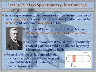
Lecture 7: Mass Spectrometry, Instrumental In mass spectrometry, components of a mixture are transferred to the gas phase (if they’re not already there) and separated by electric (and sometimes magnetic) fields. The first MS data was collected by this guy: Wilhelm Carl Werner Otto Fritz Franz Wien, 1864-1928 Wilhelm showed that ‘canal rays’ of positively charged particles could be deflected by strong Electric and Magnetic fields From this evidence, he concluded that the positively charged species responded to the EM fields based on their e/m (charge-to-mass) ratio
Mass Spectrometry: The Beginning But it was J. J. Thomson who really got things going: He improved Wilhelm’s apparatus by creating the positive rays at low pressure. As a result, we was able to separate various positive ions of gasses, and even Ne20 from Ne22 One of Thomson’s students, Francis Aston, greatly improved Thomson’s instrument The main difference was that Aston’s instrument focused ions with different speeds into a single line Francis Aston (1877-1945)
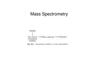
Mass Spectrometry: The Beginning At first, it looked like MS would be good mostly for analyzing isotopes. Prior to WWII, the stable isotopes of virtually every element were analyzed. After WWII, the general picture of a mass spectrometer emerged. It must have the following parts: An Ion Source – we have to get stuff into the gas phase A Mass Analyzer – we need to separate or select the desired ions A Vacuum System – we can’t have our ion beam colliding with neutrals A Detector – we need to detect our selected ions
Vacuum Systems: Roughing pumps In order to keep our ion beams focused, we can’t have them banging into neutral gasses at atmospheric pressure. In general, that means we want pressures in the 10-6 – 10-8 Torr range How do we know that? We calculate the mean free path . This is the total distance traveled in time t divided by the number of collisions: Path length (vt) Radii of colliding particles Particle density Collision cross section For small molecule gasses at ~10-7 Torr, = ~ 1000 m
Vacuum Systems: Roughing pumps Getting to 10-8 Torr ain’t easy. We need to do it in stages. The first stage uses a roughing or rotary vane pump ~10-3 Torr
Vacuum Systems: Turbo Pumps From there, we can use a turbomolecular pump: The mechanism of action is simple: The fan blades simply ‘hit’ gas molecules out of the chamber. This’ll get us down to ~10-7 Torr But what if we need to get lower?
Vacuum systems: Cryopumps Cryopumps work by trapping small amounts of gas molecules by condensing them on to a surface They have very slow pumping speeds, but can get down to ~10-12 Torr under the right conditions
Vacuum Gauges Once we have our vacuum (and while we’re making it) we need to monitor the pressure For the first pumping stage (~10-4 Torr) we can use a ‘Pirani Gauge’ Pirani gauges work by measuring the resistance through a wire exposed the vacuum. Current through the wire heats it up, exposure to surrounding gas cools it down. Conductivity is dependent on temperature. For lower stages, we usually use a Bayard-Alpert or Penning hot/cold cathode gauge . Bayard-Alpert gauges ionize residual gasses in the vacuum using a stream of electrons. The resulting positive gas ions are drawn to a negatively charged collector producing a current (1 mA/.01 Torr)
Detectors There are two major types of detectors. One, the ‘chanel electron multiplier’ (CEM) is going to look awfully familiar: The other is called a microchannel plate (MCP). And it’s basically an array of tiny CEMs. http://hea-www.harvard.edu/HRC/mcp/mcp.html
Detectors: Comparison CEM MCP Lowish Sensitivity Extreme Sensitivity Microchannels are not as efficient as dynode arrays Can easily measure a single ion Extreme Sensitivity Threshold Still have to set detection threshold quite carefully Detection threshold must be carefully set or data gets noisy! Very High Duty Cycle Low Duty Cycle Channels can return signal while others are recovering Relatively long (~500 s) recovery time Easily Saturated Easily Saturated Cannot tell the difference between lots of ions and tons of ions Cannot tell the difference between lots of ions and tons of ions
The Core: Mass Analyzers, Sector The Mass Analyzer is what makes a mass spectrometer. It’s how you select or separate ions according to their mass. The first Mass Spectrometers used sector mass analyzers, so named because ions are separated first in electric and then magnetic field sectors. To make a ‘perfect’ arc sub for v rearrange
Variations on Sector Mass Analyzers Sector instruments aren’t all that popular anymore – they’re big and clunky due to the need for a powerful magnet. But some people still use ‘em… There are a number of variations on the sector theme. One of the main advantages is the ability to focus ions in the electric (D) or magnetic sectors (E) to limit dispersion
Mass Analyzers: Quadrupoles Like sector mass analyzers, quadrupoles are mass filters: They work by letting only the desired mass through. A quadrupole mass analyzer is a set of four parallel rods:
x + y - - r0 + Quadrupole Mass Analyzers The unifying aspect of chromatographic methods is that the separation is not with an applied electric field + - - + Alternating (RF) potential Total applied potential DC potential Upon entering the quadrupole, particle will experience the following accelerations:
Quadrupole Mass Analyzers To describe the motions these forces induce, we need to sub in our equation for and differentiate with respect to x or y The trajectory of an ion is stable as long as the neither the x nor the y values reach or exceed ±r0 which corresponds to the position of one of the rods. To get the positions x and y over a timespan (residence time in the quadrupole), we would have to integrate these equations (called the Paul equations). But that would be very hard.
The Mathieu Equation So we use a trick devised by Emile Mathieu. For an oscillator, we can replace the time term t with But now we have to describe our applied potentials U and V with respect to . We can now describe the motions of our ions in the form of the Mathieu Equation:
Stability Diagrams In the Mathieu equation, r0 is constant and can be held constant. If we are interested in a particular ion (m/ze), the only variables are our applied potentials U and V, which are proportional to au andqurespectively. If we plot the stability of an ion with respect to all values of au and qu we get: We need a region that is stable with respect to U and V and x and y. The most convenient region for us is ‘A’.
Stability and Mass Selection Region ‘A’ represents a stable ion trajectory. For a given m/z, any au or qu values outside that region will cause the ion to smack into the quadrupole rods. So this is how we select ions. If we ramp up U and V proportionally so that our applied voltages pass through the smallest possible ‘tip’ of the stability area for each m/z. We can change the resolution of our mass filter by increasing our U/V slope, but we have to be careful not to miss the peak entirely!
Quadrupole Limits Resolution: Depends on residence time in quadrupole. Quadrupoles can get up to a resolution of about 5000 – but remember, in a quadrupole, higher resolution = lower sensitivity. Sensitivity: Inversely proportional to resolution Mass Accuracy: Partly depends on the precision with which you can control U and V… which is highly accurate. Around .1 Da on new instruments m/z limit: Depends on the maximum RF potential that can be applied to the quadrupole rods. Normally goes to about 7000 V. The practical limit is about 10,000 – 15,000 V for electronic and arcing reasons. 7000 V translates into a limit of about 5000 m/z.
Tandem Quadrupole MS Many mass spectrometers have quadrupoles set up in tandem for the purpose of carrying out MS/MS The most common setup is a ‘tripple quadrupole’ arrangement: Q1 Collision (Q2) Q3 High Pressure, RF only We can characterize molecules via a number of MS/MS modes: Fragment Ion Scan: Q1 Fixed, Q2 Collide, Q3 Scan Precursor Ion Scan: Q1 Scan, Q2 Collide, Q3 Fixed Neutral Loss Scan: Q1 Scan, Q2 Collide, Q3 Scan - offset
Quadrupole (Paul) Ion Traps In a Quadrupole Ion Trap, we collect ions in a 3D quadrupolar field with ‘end caps’ to control stability in the z direction End Cap Ring The normal way to get a mass spectrum from an ion trap is to ramp the end cap RF which causes steadily larger ions to be ejected in the z direction. You can also select the ion of interest by ramping Uz (down) and Vz (up), called a mass selective stability scan
Ion Trap Limits/Advantages Ion traps are capable of MSn experiments: 1. Select Ion of Interest 2. Tickle ion of interest (gently) using it’s ‘secular frequency’ 3. Allow destructive collisions with damping gas molecules 4. Return to Step 1. Repeat ad nauseum. Resolution: Depends on the number of RF cycles in the trapping field. Typically around 8,000 for new instruments. Up to 30,000 has been reported. Mass Accuracy: Like resolution, depends on the ramp-up speed of the RF ‘escape’ voltage. Around .2 Da Space/Charge Effects: Trapped ions, all like-charged, repel each other reducing trapping efficiency and, effectively, the dynamic range of the instrument.
Time-of-Flight (TOF) Mass Analyzers In TOF mass analyzers, ions are accelerated down a long flight tube via a brief ‘pulse’ electric field Ions enter the flight tube close to a square electric pulse generator called the pusher. This imparts a potential energy zU to a charged particle which we assume is all converted to kinetic energy: Since: Rearrange
TOF Limits/Advantages The primary advantage of TOF analyzers is their max m/z, which is theoretically unlimited. Practically speaking, though, they go up to about 15,000 – a huge advantage for studying large proteins TOFs must use MCP detectors because ions of different masses hit the detector in rapid succession. This results in a very high duty cycle (mass spectra from 100 – 10,000 can be acquired in a second or less) but low sensitivity. Resolution: Dependent on the length of the TOF tube. Many TOF instruments permit a ‘W mode’ scan which effectively doubles the length, but at a price of sensitivity. TOFs can go up to 17,000 in W mode and about 11,000 in V mode. Mass Accuracy: Depends ability to generate a very square pusher pulse and measure accurate ‘arrival times’. Around .2 Da
Fourier Transform Ion Cyclotron Resonance Fourier Transform Ion Cyclotron Resonance (FT-ICR) is the highest resolution mass analyzer available. FT-ICR instruments use a strong magnetic field to cause ions to go into a circular orbit inside a set of four charged plates Trapping plate (+ve) X = H (into page) Trapping plate (+ve) The size of the orbit is defined by the same factors that made the ‘arc’ in sector instruments:
FT-ICR We can measure m/z this way because the angular velocity of the ions is dependent on their mass: Since v = r… How do we measure c? We do it by detecting the tiny current induced by the ions as they pass close to the plates receiver plate Our signal… receiver plate
Putting the ‘FT’ in FT-ICR So our data is in the ‘time domain’, meaning that we are looking at our signal as a function of time. But we’re interested in frequency. We’ve seen this before and we know what we have to do. Over time, our cloud of ions will loose coherence due to collisions with gas, ion/ion repulsion etc. This will make our time domain signal decay exponentially. Frequency Domain Time Domain FT
Tickling Ions in FT-ICR When ions enter the FT-ICR cell, they will have very small orbital radii – so they’re not near the receiver plates – and their motion isn’t coherent – particles with the same m/z are not ‘bunched together’. The solution is similar to a quadrupole ion trap: We ‘tickle’ ions at their orbital frequency c by applying an additional RF potential to the trapping plates. This will solve both of the above problems at once. We can either select ions by using a specific RF frequency (this is used to excite ions for fragmentation or eject undesired ions) or… We can use a reverse FT to figure out what RF signal we need to excite a range of frequencies (this is used to collect mass spectra)…
Getting Mass Spectra with FT-ICR Lets say we want to excite ions oscillating at c of 1-5. We need an excitation profile something like this: Now we need to figure out what excitation signal will give us this excitation profile: invFT And now we apply that RF profile to the plates. This is called Stored Waveform Inverse Fourier Transform (SWIFT)
FT-ICR = The Best Mass Analyzer! Apart from being very expensive, FT-ICRs are the best kind of Mass Analyzer. Here’s why: Resolution: Frequencies can be measured very accurately. And in FT-ICR those frequencies can be measured over and over with multiple excitation pulses. FT-ICRs regularly get resolutions in the 106 range. Sensitivity: Currents induced by the cycling ions may be weak, but they can be amplified. FT-ICR cells can detect as little as one ion! and can store up to ~105! Mass Accuracy: Can be very good (.01 Da) with careful calibration Duty cycle: Pretty quick. Mass Spectra are collected in milliseconds to seconds.
Ion Sources The mass analyzer may make the mass spectrometer, but it is advances in ion generation methods that have made MS suitable for biological applications. Since we’re concerned with analytical biochemistry, we’re going to skip over the following ways of making ions: Chemical Ionization (CI) – ions from collisions with reagent gas Fast Atom Bombardment (FAB) – sample is hit with a stream of H+, producing secondary ions Inductively Coupled Plasma (ICP) – sample is passed through a plasma ‘flame’ Electron Impact/Ionization (EI) – ions from collisions with electrons
MS for Biomolecules There is one main ionization process requirement for the analysis of biological molecules by MS: It needs to be gentle. We want to see intact biological macromolecules. ½ of the 2002 Nobel prize in chemistry was for the invention of soft ionization techniques: Koichi Tanaka John Fenn Matrix Assisted Laser Desorption Ionization (MALDI) Electrospray Ionization (ESI)
Matrix Assisted Laser Desorption Ionization In MALDI, a laser is used to irradiate a sample that is embedded in a matrix The Matrix is usually a small organic molecule that is good at forming crystals and absorbs light at the irradiation wavelength. MS
MALDI Ionization Ions formed by MALDI can be of the ‘primary’ or ‘secondary’ variety. Primary (probably matrix molecules): Secondary (matrix or analyte molecules, this occurs in the MALDI ‘plume’): Excited State Proton Transfer Gas Phase Proton Transfer The above mechanisms are probably most applicable to biological analytes, but there are plenty of other ways that ions can form!
Ions from MALDI So the predominant mechanism for analyte ion formation is just a proton transfer, which would be quite gentle. We just have to make sure our laser won’t destroy our analyte, which is unlikely in any case, but it helps to pick a wavelength at which the analyte doesn’t absorb (for proteins and peptides, usually around 300 nm). Other important considerations: Gas phase transfer is not great at making multiply charged ions. Thus m/z will be quite high. We will need a TOF mass analyzer… MALDI is actually more efficient at ionizing the matrix than the analyte. Consequently the ‘low mass’ region of MALDI spectra will be washed out by matrix and matrix fragmentation products
Droplet shrinkage + + + + + +5 kV + + + + + + + + + + + + Taylor cone + + Electrospray Ionization (ESI) In electrospray, ions are formed by passing a solution containing your analyte through a capillary that is held at a high potential We’re not sure how the final step works. Could be the ion evaporates out of the tiny droplet (ion evaporation model, IEM), or the solvent continues to evaporate, leaving a ‘charge residue’ on the analyte (charged residue model, CRM) – or could be both.
ESI Characteristics and Advantages ESI is be carried out a atmospheric pressure. Ions are transported into the mass spectrometer via a differentially pumped interface. ESI is carried our from bulk solution. No need for ‘mixing with matrix and drying’ steps. This makes ESI ideal for coupling with LC purification/ separation ESI is very good at producing multiply charged ions. Thus, even very big, heavy things can be analyzed ESI is gentler than a baby’s handshake. It’s so gentle that even non-covalent protein complexes can be transferred intact into the gas phase. ESI is not tolerant to non-volatile salts… such as those used by biochemists (e.g. NaPO4)
ESI and Charge State Distributions For a single protein, ESI will almost always generate several charge states. The intensities of these charge states are arranged in a roughly Gaussian distribution (although there is no physical justification for this). This is called the charge state distribution. We can look at a raw protein mass spectrum (intensity vs. m/z) and deconvolute it to a single mass using the formula: Mass of charge imparting ‘adduct’ (usually H+) Mass of analyte Number of charges
Charge State Distributions and Protein Folding Importantly, the charge state distribution reflects the folding state of the protein - Low charge - Tight distribution I - Probably Folded m/z - High Charge - Wide distribution I - Probably unfolded m/z