A Core Course on Modeling
A Core Course on Modeling. Week 4-Dealing with mathematical relations. From graph shape to functional relation . 1. A taxonomy on the basis of graph shapes assume functions f: R R focus on behavior for x ‘in the long run’ (x and x - , or as far as they get )

A Core Course on Modeling
E N D
Presentation Transcript
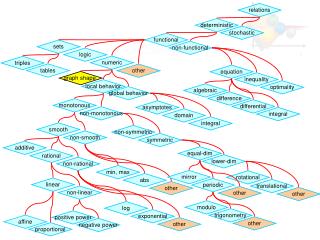
A Core Course on Modeling Week 4-Dealing with mathematical relations From graph shape to functional relation 1 • A taxonomy on the basis of graph shapes • assume functions f:R R • focus on behavior for x ‘in the long run’ (x and x - , or as far as they get) • heuristic: no guarantee for ‘correctness’ • may need a bit of tuning to get the right parameterization • start with searching a match with few as possible parameters • experiment!
A Core Course on Modeling Week 4-Dealing with mathematical relations From graph shape to functional relation 2
A Core Course on Modeling Week 4-Dealing with mathematical relations From graph shape to functional relation 3 Behavior Suggested parameterisation Parameters How to fit Example Remarks Linear y = ax + b a: slope with the +x axis; b: intercept with the y-axis linear least squares (http://en.wikipedia.org/wiki/Linear_least_squares_(mathematics) ); The world record time on 100 m sprint as a function of time (this example shows the limitations of extrapolating simple models; see Edwards & Hamson, page 10 and further)
A Core Course on Modeling Week 4-Dealing with mathematical relations From graph shape to functional relation 4 Behavior Suggested parameterisation Parameters How to fit Example Remarks Piecewise linear (tent- or V-shape, sharp bend) y = a abs(x - x0) + b a: slope with the +x axis; b: height of the apex; x0 : location of the (+ or -) apex first estimate x0; next linear least squares to find a and b (http://en.wikipedia.org/wiki/Linear_least_squares_(mathematics) ); Accurate measurements using compensation method (e.g., Wheatstone bridge for measuring resistance, capacity, inductance) Possibly the slopes of left- and right segments are too different; then: treat as two separate lines
A Core Course on Modeling Week 4-Dealing with mathematical relations From graph shape to functional relation 5 Behavior Suggested parameterisation Parameters How to fit Example Remarks Horizontal asymptote left (right); unbounded increase/decrease right (left) or vice versa y = exp (b (x-x0)) + a a determines the height of the asymptote; the sign of b determines which side (left or right) the asymptote; x0 determines the rate of increase/decrease first estimate a; next take log(y-a) =b(x-x0) and estimate b and x0 using linear least squares. Proportional growth, e.g. financial assets (compound interest), populations; absorption in a medium (x=thickness), radioactive decay (x=time), … Alternative parameterisation: y = y0 exp bx + a
A Core Course on Modeling Week 4-Dealing with mathematical relations From graph shape to functional relation 6 Behavior Suggested parameterisation Parameters How to fit Example Remarks Vertical asymptote left (right); unbounded increase/decrease right (left) or vice versa y = a log (b (x-x0)), b(x-x0) >0 x0 determines the location of the asymptote; the sign of a determines increase or decrease; the sign of b determines whether increase/decrease is for ascending or descending x. first estimate x0; next set x-x0 t and plot y against exp(t): y=a(log b+t). Linear least squares gives a and slope=a log b. Find b as exp(slope/a).. Perception (e.g., perceived loudness is proportional to the log of the air pressure); computing science (execution time of algorithms sometimes grows proportional with log of data size) Alternative parameterisation: y = y0 +log(x-x0), x>x0 or y0+log(x0-x), x<x0
A Core Course on Modeling Week 4-Dealing with mathematical relations From graph shape to functional relation 7 Behavior Suggested parameterisation Parameters How to fit Example Remarks Unbounded increase left, decrease right – or vice versa y = a x2 + b x + c a determines curvature; b left-right symmetry; c absolute height. first estimate apex (xa,ya); find point (xa+p,yshift) for arbitrary p. Then a = (yshift-ya)/p2; b = -2axa; c = ya+b2/4a Free falling and thrown objects have parabolic trajectories; stopping distance for braking cars is quadratic in speed; air resistance on a moving object is (roughtly) parabolically dependent; potential energy for an oscillating system; area of a surface given a characteristic dimension. Any even degree polynomial has the behavior of unbounded increase or decrease both left and right; they can have inflection points and therefore multiple local extrema. For large |x|, only the highest power dominates, so left branch and right branch tend to be mirror symmetric for large |x|.
A Core Course on Modeling Week 4-Dealing with mathematical relations From graph shape to functional relation 8 Behavior Suggested parameterisation Parameters How to fit Example Remarks Asymptotic increase left, decrease right – or vice versa y=a+b tan 2 (c(x-x0)) The location of the asymptotes determines c and x0 The height of the apex is a; b determines the steepness. Let xa1 and xa2 the locations of the asymptotes. Then x0=(xa1+xa2)/2; c=/(xa2-xa1). The height of the apex is a; b tunes the steepness. No known examples.
A Core Course on Modeling Week 4-Dealing with mathematical relations From graph shape to functional relation 9 Behavior Suggested parameterisation Parameters How to fit Example Remarks Unbounded increase (decrease) left and right – monotonically or not y = a x3 + b x2 + c x + d or Brute-force method: substitute at least 4 points (xi,yi) into y=ax3+bx2+cx+d and solve linear set of equations for a,b,c,d in least-squares sense. For all coefficients ≠0: no common applications known. For only a ≠ 0: the volume or the mass of an object, given its characteristic dimension. Although the cubic function (or higher, odd-degree polynomial functions) have little practical application, cubic parameter curves x=Fx(t), y=Fy(t) , 0t 1 (so called splines) form the working horse of most of computer aided geometric design: since they have 4 parameters, they can satisfy two continuity constraints on both ends (values and tangents), and form a smooth curve consisting of piecewise cubic curves.
A Core Course on Modeling Week 4-Dealing with mathematical relations From graph shape to functional relation 10 Behavior Suggested parameterisation Parameters How to fit Example Remarks Asymptotic increase (decrease) left and right y = c tan (a(x-b))+d a and b shift the curve to the left or the right; a and c together determine the steepness in the inflection point; d is a vertical offset First find a and b such that asymptotes are on the right locations, use that tan(x) has asymptotes for /2 and -/2. Next adjust c to get the steepness right; finally adjust d to get the intersection with x-axis right. tan functions often occur in relation to geometric problems involving angles or ratios of lengths. E.g., find the height of a building from the length of its shadow and the angle of the sun above the horizon. An alternative parameterization is, for instance, y = x/((x-x0)(x-x1)). This function has two vertical asymptotes, for x=x0 and x1 respectively. However, it also has horizontal asymptotes; in our taxonomy it would therefore classify as ‘saturation both left and right, increasing or decreasing everywhere’
A Core Course on Modeling Week 4-Dealing with mathematical relations From graph shape to functional relation 11 Behavior Suggested parameterisation Parameters How to fit Example Remarks Asymptotic decrease left, saturating increase right – or vice versa several; simplest in use: y = c((a/x)12-2(a/x)6) c is a scale factor, determining the depth of the ‘dip’; a is the x-value for which the minimum is reached. Find the location of the dip; its x-coordinate is a. Next substitute the y value of the minimum to adjust c. The force between particles (atoms, molecules) if often a combination of attraction at long distance andd repulsion at short distance. This form for the interaction was proposed by, and named after E. Lennard-Jones. http://en.wikipedia.org/wiki/Lennard-Jones_potential
A Core Course on Modeling Week 4-Dealing with mathematical relations From graph shape to functional relation 12 Behavior Suggested parameterisation Parameters How to fit Example Remarks Linear increase left, saturating decrease right – or vice versa y = C x * logistic curve (x) C is overall scale factor; should be 1 if x and y are in same units.Logistic curve can have various parameterizations. Find overall scale factor C from slope left hand part; next divide by Cx and find parameters for logistic curve as described with logistic curve. Income as a function of selling price: if the price is to low, income is low despite large volume; if the price is too high, market (share) will be too small. There are no immediate interpretations of the curve with x -x of with y -y.
A Core Course on Modeling Week 4-Dealing with mathematical relations From graph shape to functional relation 13 Behavior Suggested parameterisation Parameters How to fit Example Remarks saturation both left and right, increasing or decreasing everywhere. When monotonous, a logistic curve is a likely candidate. in standard form: y=1/(1+exp(-x)) Standard version has no parameters: asymptotes for y=0 and y=1. Standard inflection point for x=0 and slope 1. For arbitrary asymptotes, inflection point and slope, use Richards generalised logistic curve; see http://en.wikipedia.org/wiki/Generalised_logistic_curve Applications in ecology (population growth), chemistry (autocatalyse), neural networks, medicine (tumor growth), physics (Fermi distribution), economy (price elasticity) Depending on the application, other parametrizations can be y=a arctan (bx +c)+d, or piecewise linear (ramp function) . If the function can have a vertical asymptote (that is, is not monotonous), a two-branch hyperbola like y = 1/x could be tried.
A Core Course on Modeling Week 4-Dealing with mathematical relations From graph shape to functional relation 14 Behavior Suggested parameterisation Parameters How to fit Example Remarks saturation left or right, and a vertical asymptote; monotonically increasing or decreasing. one branch of an (orthogonal) hyperbola y=a+b/(x-c) a and c define asymptotes; b defines slope. Find vertical asymptote; this defines c. Find horizontal asymptote; this defines a. Slope is controlled by b; sign of b defines which the quadrants. In physics, the product of P and V (pressure and volume) for an amount of gas with constant temperature is constant. Both are non-negative, so only one branch of the hyperbola.
A Core Course on Modeling Week 4-Dealing with mathematical relations From graph shape to functional relation 15 Behavior Suggested parameterisation Parameters How to fit Example Remarks monotonically increasing or decreasing with inflection point, no saturation y=x 1/3 Characteristic dimension of an object with volume x Compare with y=x1/2=xon;y defined for x>0. Applications of square root: mechanics (fall time of a point mass for given height); applications involving Pythagoras’ theorem; characteristic dimension of a surface with given area.
A Core Course on Modeling Week 4-Dealing with mathematical relations From graph shape to functional relation 16 Behavior Suggested parameterisation Parameters How to fit Example Remarks saturation both left and right, approached from the same side; (1) no vertical asymptotes y=a exp (-(x-b)2/2c2) (Gaussian), or y = a / (1+(x-b)2/2c2) (Lorentzian) b is location of maximum; c relates to width of half maximum; a is height of maximum. Gaussian: statistics, normal distribution; Lorentzian: distribution of energy in spectra, forced resonance; geometric distribution of light from a point source over a surface. The Lorentzian has a ‘thicker’ tail than the Gaussian. It counts as a pathological distribution in statistics, because it has no mean and its variance is infinity.
A Core Course on Modeling Week 4-Dealing with mathematical relations From graph shape to functional relation 17 Behavior Suggested parameterisation Parameters How to fit Example Remarks saturation both left and right, approached from the same side; (2) vertical asymptote y = 1 / ((x-b)2/2c2) b is location of vertical asymptote; c relates to width of peak Distribution of light from a point source over a surface containing the light source

