Nested Designs
Nested Designs. Study vs Control Site. Nested Experiments. In some two-factor experiments the level of one factor , say B, is not “cross” or “cross classified” with the other factor, say A, but is “NESTED” with it. The levels of B are different for different levels of A.


Nested Designs
E N D
Presentation Transcript
Nested Designs Study vs Control Site
Nested Experiments • In some two-factor experiments the level of one factor , say B, is not “cross” or “cross classified” with the other factor, say A, but is “NESTED” with it. • The levels of B are different for different levels of A. • For example: 2 Areas (Study vs Control) • 4 sites per area, each with 5 replicates. • There is no link from any sites on one area to any sites on another area.
Study Area (A) Control Area (B) S1(A) S2(A) S3(A) S4(A) S5(B) S6(B) S7(B) S8(B) X X X X X X X X X X X X X X X X X X X X X X X X X X X X X X X X X X X X X X X X X = replications Number of sites (S)/replications need not be equal with each sites. Analysis is carried out using a nested ANOVA not a two-way ANOVA. • That is, there are 8 sites, not 2.
A Nested design is not the same as a two-way ANOVA which is represented by: A1 A2 A3 B1 X X X X X X X X X X X X X X X B2 X X X X X X X X X X X X X X X B3 X X X X X X X X X X X X X X X Nested, or hierarchical designs are very common in environmental effects monitoring studies. There are several “Study” and several “Control” Areas.
Objective • The nested design allows us to test two things: (1) difference between “Study” and “Control” areas, and (2) the variability of the sites within areas. • If we fail to find a significant variability among the sites within areas, then a significant difference between areas would suggest that there is an environmental impact. • In other words, the variability is due to differences between areas and not to variability among the sites.
In this kind of situation, however, it is highly likely that we will find variability among the sites. • Even if it should be significant, however, we can still test to see whether the difference between the areas is significantly larger than the variability among the sites with areas.
Statistical Model Yijk = m + ri + t(i)j + e(ij)k i indexes “A” (often called the “major factor”) (i)j indexes “B” within “A” (B is often called the “minor factor”) (ij)k indexes replication i = 1, 2, …, M j = 1, 2, …, m k = 1, 2, …, n
Model (continue) Or, TSS = SSA + SS(A)B+ SSWerror = Degrees of freedom: M.m.n -1 = (M-1) + M(m-1) + Mm(n-1)
Example M=3, m=4, n=3; 3 Areas, 4 sites within each area, 3 replications per site, total of (M.m.n = 36) data points M1 M2 M3Areas 1 23 45678 9101112 Sites 10 12 8 13 11 13 9 10 13 14 7 10 14 8 10 12 14 11 10 9 10 13 9 7 Repl. 9 10 12 11 8 9 8 8 16 12 5 4 11 10 10 12 11 11 9 9 13 13 7 7 10.75 10.0 10.0 10.25
Example (continue) SSA = 4 x 3 [(10.75-10.25)2 + (10.0-10.25)2 + (10.0-10.25)2] = 12 (0.25 + 0.0625 + 0.625) = 4.5 SS(A)B = 3 [(11-10.75)2 + (10-10.75)2 + (10-10.75)2 + (12-10.75)2 + (11-10)2 + (11-10)2 + (9-10)2 + (9-10)2 + (13-10)2 + (13-10)2 + (7-10)2 + (7-10)2] = 3 (42.75) = 128.25 TSS = 240.75 SSWerror= 108.0
ANOVA Table for Example Nested ANOVA: Observations versus Area, Sites Source DF SS MS F P Area 2 4.50 2.25 0.158 0.856 Sites (A)B 9 128.25 14.25 3.167 0.012** Error 24 108.00 4.50 Total 35 240.75 What are the “proper” ratios? E(MSA) = s2 + V(A)B + VA E(MS(A)B)= s2 + V(A)B E(MSWerror) = s2 = MSA/MS(A)B = MS(A)B/MSWerror
Summary • Nested designs are very common in environmental monitoring • It is a refinement of the one-way ANOVA • All assumptions of ANOVA hold: normality of residuals, constant variance, etc. • Can be easily computed using MINITAB. • Need to be careful about the proper ratio of the Mean squares. • Always use graphical methods e.g. boxplots and normal plots as visual aids to aid analysis.