Download
1 / 67
670 likes | 698 Vues
Explore the simulation vs. animation, known vs. unknown, and scientific vs. fictional aspects of fundamental parameters and calculations in Density Functional Theory. Discover the advantages, limitations, and applications of this groundbreaking theory.

E N D
Ab-initioDensity Functional Theory:from quantum dots to solar cell SaiffulKamaluddinMuzakir Staf ID: 01009 019 276 3844 skmuzakir@yahoo.com www.facebook.com/Saifful Kamaluddin
Simulation vs animation Result Unknown Known Scientific based Fundamental Fiction/imaginary Fundamental parameter Input Script/ storyboard Calculation Simple or none Complicated Eq.’s accuracy dependency Realistic Script’s dependency Predict results Usage Tell results Investigative Technologies Inc.
The advantages of simulation wet lab Cluster size Excited state Ground state Electron density Absorption spectroscopy IR spectroscopy
Ab initio Crystallographic profile, number of electrons, neutrons, protons • Maths • functions & functionals Dr. Izan Material properties 1 2 ….. 1,000,000 OUTPUT Experimental data
Function y = f(x) = 2x+3 “y is a function of x” OUTPUT y Vito Volterra “Theory of functionals and of Integral and Integro-Differential Equations”(1930)
Functional z = g(x)+h(x)-i(x) i(x)=x+2 h(x)=4x g(x)=2x “z is a functional of x” OUTPUT z
Density Functional Theory ρ ρ ρ ρ electron density, ρ ρ ΣE= Σ(K.E)+ Σ(P.E) P.En-n P.Ee-e P.Ee-n K.Ee Exc K.En “Total ground state energy of a system is a functional of electron density” OUTPUT Total Ground State Energy
From Schrödinger’s equation to DFT Predicts the evolution behaviour of a dynamic system • Mathematical function that describe a system in the form of summation of K.E & P.E Determine by Basis set Determine by Functional
DFT evolution • Early DFT (1970s): • Hψ= Eψ • (ΣE)ψ=(ΣK.E + ΣP.E)ψ =(K.Enuc+ K.Eelec. +P.En-n +P.Ee-n +P.Ee-e)ψ • Modern DFT (1990s): (ΣE)ψ=[K.Eelec. + P.Ee-n + P.Ee-e + Exc]ψ • (ΣE)ψ=[K.Ee(ρ)+ P.Ee-n(ρ)+ P.Ee-e(ρ)+ Exc(ρ)]ψ Nucleus is heavy and ~static: K.E= ~0 Nucleus is neutralized:
Basis set & Functional (model) • Basis set: • Set of wavefunction, ψ • Shape of each atom’s orbitals (AOs) • Calculations with approximations & corrections • Functional: • System modeling, H • Molecular Orbitals (MOs) • Energy (Warren J. Hehre. Wavefunction Inc. 1996) (Errol G. Lewars, 2011)
Choice of functional DISCLAIMER: The accuracy of results also heavily depends on the basis set used! Accuracy Increases ions, excited state… Same orbital spatial functions for all electrons UHF Accuracy Increases Ab initio: HF RHF Different functions Semi empirical (G09 W) paired e- species DFT: B3LYP PM3 ZINDO Etc.. There other models not listed. Here are the most common MORE FUNCTIONAL DETAILS:http://www.gaussian.com/g_tech/g_ur/k_dft.htm
Limitation of basis set CdSe http://www.gaussian.com/g_tech/g_ur/m_basis_sets.htm
Basis set choices Narrow down choices: by limitation Literature review: Any previous theoretical work? NO Produce own experimental results YES NO Realistic molecular/cluster model Use the same basis set Use all short-listed basis sets YES Simulate results Comparison with previous experimental work. Any published work?
Basis set accuracy:comparison with experimental data List of basis set: http://www.gaussian.com/g_tech/g_ur/m_basis_sets.htm
Application: Quantum dot solar cell Working electrode Counter electrode TiO2 Quantum dot Ligand Ligand Ligand e- e- Ligand TiO2 Ligand Ligand Ligand e- e- Electrolyte e- e- A. Electron injections:Is it POSSIBLE & EFFICIENT? QD Ligand B. Ligand-QD adsorptionIs it POSSIBLE & HOW STRONG?
Series of simulation PROCESSES RESULTS INPUT Structure optimization Optimization of:Bond length, Angle and Dihedral angle With estimated parameters (to be optimized) Frequency simulation Positive vibrational frequency: A realistic molecular/cluster model Energy calculation Energy: Ground state & excited state Full population simulation Visualization of excited and ground state’s electron density Size calculation Size of modeled molecule/cluster
Input preparations • Input: • Molecules (i.e., ligand molecules) • Quasi-Crystals (Quantum dots semiconductor) • Drawing Tools: • ChemDraw • Chem3D • Gaussview • Ab initio DFT Tool: Gaussian 09W
Input: Ligand molecule What is a molecule? A group of atomsbonded together, representing the smallestfundamental unit of a chemical compound that can take part in a chemical reaction A single molecule can represents a system consists of ten/hundreds/thousands/millions/billions of them Merriam-Webster Dictionary
Molecule Input Step 1: Draw molecule Draw using Chemdraw HS HS Save As *.mol2 O O O O Select All, Grab & Drag to OH OH HO HO Chemdraw 3D & release
Molecule Input Step 2: Labeling molecule Open *.mol2 file using Gaussview 5.0 1. Right click2. Select “View”
Molecule Input Step 3: Rearrange numbers • Click “edit” – “Atom list” • A new interface appears: showing labels. Rearrange the numbers in a nice flow. Computer generated Z-Matrix:Pro: Can be straight away use as simulation input.Con: Tested & may cause longer simulation time.Solution: Spend time building our own Z-Matrix Before & After
Molecule Input Step 4: Building z-matrix • Define all atoms using: • Bond length • Angle • Dihedral angle • 1H need no definition: starts from here • 2O is connectedto 1H by A BOND • 3C is connected to 2O by A BOND is bent from 1H by AN ANGLE • 4O is connected to 3C by A BOND is bent from 2O by AN ANGLE is twisted from 1H by a DIHEDRAL ANGLE • 5C is…next slide
Molecule Input Step 5: Defining bond, angle & dihedral angle 5C 3C • 5C is connected to by a bond is bent from by an angle is twisted from by a dihedral angle 2O 1H 5C 5C 3C 3C 2O 2O 1H 1H 3C ? 2O ? 1H ?
Molecule Input Step 6: Z-matrix, the format H O 1 B1 C 2 B2 1 A1 O3 B3 2 A2 1 D1 1H 2O is connectedto 1H by A BOND 3C is connected to 2O by A BOND is bent from 1H by AN ANGLE 4O is connected to 3C by A BOND is bent from 2O by AN ANGLE is twisted from 1H by a DIHEDRAL ANGLE A description of an atom must be: In 1 LINE Each line is meant for 1 atom’s description ONLY May use any symbol for bond, angle and dihedral B1, B2, A1…D1….must be stated as simulation parameters and the value will be optimized OR as CONSTANTi. stated in DECIMAL POINT as INDICATION of CONSTANT, i.e., 1.546 ii. stated in the form of 1. ONLY as INDICATION of TO BE OPTIMIZED (Will show the full format later)
Molecule Input Step 7: Estimating bond length H O 1 B1 C 2 B2 1 A1 C3 B3 2 A2 1 D1 If we want to: (a) Make it as constant, change B1 with “0.96” in the Z-Matrix (b) Optimize the value, write “B1=1.”
Molecule Input Step 8: Estimating angle H O 1 B1 C 2 B2 1 A1 C3 B3 2 A2 1 D1 B2=1.43 A1=109.47122
Molecule Input Step 9: Estimating dihedral angle H O 1 B1 C 2 B2 1 A1 C3 B3 2 A21 D1 B3=1.2584 A2=120.0 D1=30.0
Molecule Input Step 10: Full Z-Matrix FULL Z-MATRIX • TEST the z-matrix: • Open Gaussian 09W • Click “File” & “New” • Key in %section,route section and title as indicated • Copy & Paste the Z-matrix in the “Molecule Specification” field • Save Job As….(any name) • Open the file using Gaussview 5.0 • If the Z-Matrix is CORRECT, it will show the same molecule model as the reference
Molecule Input: Done Build reference molecule Gaussview Chemdraw Building z-matrix From 2D to 3D Build Z-matrix Word processing Gaussview Write down z-matrix Rearrange labels Z-matrix testing REFINE THE MODEL:Check Z-matrix and Gaussian setting Gaussian Key in setting, z-matrix & save the MODEL Is the model similar to the reference molecule? YES ERROR/NO RUN the simulation on Gaussian WHICH PROCESS?
Molecule Series of simulation PROCESSES RESULTS INPUT Structure optimization Optimization of:Bond length, Angle and Dihedral angle With estimated parameters (to be optimized) Frequency simulation Positive vibrational frequency: A realistic molecular/cluster model Energy calculation Energy: Ground state & excited state Full population simulation Visualization of excited and ground state’s electron density Size calculation Size of modeled molecule/cluster
Molecule %Section field
Molecule %Section field • The directory to save “.chk” file (a file that records all calculations, achievable at any simulation process by using “check” command in “Route Section”):%chk= C:\g09w\PbTe.chk • Stating the amount of memory usage in MW (megawords). 1 MW=3.81 MBytes%mem=200MW
Molecule Route Section field
Molecule Route Section 1: Geometry opt. • Stating the command line of simulation: • # opt b3lyp/lanl2dz direct optcyc=100 Functional Basis set Max number of optimization No calculation storage required (faster process) Geometry optimization command Job initiation
Molecule Route Section 2: Frequency • Stating the command line of simulation: • #n b3lyp/lanl2dz direct freqgeom=check guess=check Default:Normal print level of output Retrieve molecular orbitals data from “.chk” file (previous geometry opt.) Frequency command Retrieve internal coordinate from “.chk” file (previous geometry opt.) Without “geom=check” and “guess=check” command: Have to state “Optimized Z-matrix” in the “Molecule Spec” field
Molecule Route Section 3: Energy • Stating the command line of simulation: #n b3lyp/lanl2dz direct TD (direct, singlet, root=1, Nstates=50)geom=check guess=check Number of each type of state to be solved. Default=3 Time dependent Singlet excited state State of interest. Default is 1 (first excited state)
Molecule Route Section 4: Full population • Stating the command line of simulation: #n b3lyp/lanl2dz pop=full geom=check guess=check Molecular orbitals visualization, total atomic charge and orbital energies
Molecule Route Section 5: Cluster size estimation • Stating the command line of simulation: #p b3lyp/lanl2dz scrf=pcmgeom=check • Choices of solvent (to be specified in command line): http://www.gaussian.com/g_tech/g_ur/k_scrf.htm Calculate volume & surface area of cluster in solution. Default: Water Use with energy, geometry opt, freqcalc to model systems in solution Additional output (execution timing, messages etc)
Molecule Charge & Multiplicity
Molecule Charge & multiplicity • Charge: total charge of the molecule OR cluster = 0
Molecule Charge & multiplicity • Multiplicity/spin multiplicity: describes how the electrons of the system exist • 2S+1=spin multiplicity, where S is total spin quantum number • S=n(1/2) where n=unpaired electron S H H H H O O mercaptosuccinic acid molecule Inorganic Chemistry J.E. House, Academic Press 2008 O O H H
Molecule The rough model: mercaptosuccinic acid C C S O O C S C H H H H H H H H O O C C H O O C C UNPAIRED ELECTRON, n=0 Spin multiplicity, 2S+1=2(n(1/2))+1=2(0)+1=1 H H H O O
Molecule Running the simulation Click RUN Pop up message: specifying output directory Specify *.chk directory & memory Command line Your desired title Molecule/cluster charge & spin multiplicity Molecule/cluster’s Z-Matrix
Molecule Extracting result:Structure optimization Optimization complete Double click the output Frequency simulation Open in Gaussview Energy calculation Work doesn’t kill, But worry does -unknown post graduate student Save as Gaussian Input Files (.gjf) Full population simulation Input for NEXT SIMULATION Size calculation
Molecule Input for Frequency, Energy, Full Population & Size Open Gaussian Click File Click Open Select the saved “Structure optimization output” which saved as .gjf A new interface appears (as shown) Change “Route Section” to frequency/energy/full population/size command Leave “Molecule Specification” blank Click RUN Specify output directory
Molecule Analyzing result:Frequency simulation Completed Freq. simulation Double click the output Open in Gaussview REALISTIC MOLECULAR MODEL:Positive frequencies
Molecule Analyzing result:Energy simulation Completed Energy calculation Double click the output Open in Gaussview Absorption curve Oscillator strength
Molecule Analyzing result:Full Population Completed Full Population Double click the output LUMO Open in Gaussview HOMO Excited state energy, LUMO=-0.14320 H x 26.211=-3.753 eV Ground state energy, HOMO: -0.26601 H x 26.211=-6.972 eV
Molecule Analyzing result:Molecule size Completed Size calculation Double click the output Surface area (sphere)= 4πr2 197.708 Å2 = 12.568 r2 r = 3.966 Å d = 7.932 Å Open in Gaussview
Crystal Input: QD semiconductor • BULK semiconductor: • Crystal • Bond length, angle and dihedral angle are constant • QUANTUM DOT semiconductor: • Quasi-crystal • Bond length, angle & dihedral anglechange due to surface relaxations • FULL OPTIMIZATION (bond length, angle & dihedral) Puzder et al Phys. Rev. Lett. 92, 217401 (2004) Self-Healing of CdSeNanocrystals: First-Principles Calculations