CS 691 Computational Photography
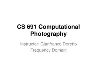
CS 691 Computational Photography. Instructor: Gianfranco Doretto Frequency Domain. Overview. Frequency domain analysis Sampling and reconstruction. Linear image transformations. In analyzing images, it’s often useful to make a change of basis. transformed image. Vectorized image.

CS 691 Computational Photography
E N D
Presentation Transcript
CS 691 Computational Photography Instructor: Gianfranco Doretto Frequency Domain
Overview • Frequency domain analysis • Sampling and reconstruction
Linear image transformations • In analyzing images, it’s often useful to make a change of basis. transformed image Vectorized image Fourier transform, or Wavelet transform, or Steerable pyramid transform
Self-inverting transforms Same basis functions are used for the inverse transform U transpose and complex conjugate
Salvador Dali “Gala Contemplating the Mediterranean Sea, which at 30 meters becomes the portrait of Abraham Lincoln”, 1976 Salvador Dali, “Gala Contemplating the Mediterranean Sea, which at 30 meters becomes the portrait of Abraham Lincoln”, 1976 Salvador Dali, “Gala Contemplating the Mediterranean Sea, which at 30 meters becomes the portrait of Abraham Lincoln”, 1976
A nice set of basis Teases away fast vs. slow changes in the image. This change of basis has a special name…
Jean Baptiste Joseph Fourier (1768-1830) ...the manner in which the author arrives at these equations is not exempt of difficulties and...his analysis to integrate them still leaves something to be desired on the score of generality and even rigour. had crazy idea (1807): Anyunivariate function can be rewritten as a weighted sum of sines and cosines of different frequencies. • Don’t believe it? • Neither did Lagrange, Laplace, Poisson and other big wigs • Not translated into English until 1878! • But it’s (mostly) true! • called Fourier Series • there are some subtle restrictions Laplace Legendre Lagrange
A sum of sines Our building block: Add enough of them to get any signal f(x) you want!
Frequency Spectra • example : g(t) = sin(2πf t) + (1/3)sin(2π(3f) t) = +
Frequency Spectra = + =
Frequency Spectra = + =
Frequency Spectra = + =
Frequency Spectra = + =
Frequency Spectra = + =
Fourier basis for image analysis Intensity Image Frequency Spectra http://sharp.bu.edu/~slehar/fourier/fourier.html#filtering
Signals can be composed + = http://sharp.bu.edu/~slehar/fourier/fourier.html#filtering More: http://www.cs.unm.edu/~brayer/vision/fourier.html
Fourier Transform • Fourier transform stores the magnitude and phase at each frequency • Magnitude encodes how much signal there is at a particular frequency • Phase encodes spatial information (indirectly) • For mathematical convenience, this is often notated in terms of real and complex numbers Amplitude: Phase: Euler’s formula:
Computing the Fourier Transform Continuous Discrete k = -N/2..N/2 Fast Fourier Transform (FFT): NlogN
Fourier transform of a real function is complex difficult to plot, visualize instead, we can think of the phase and magnitude of the transform Phase is the phase of the complex transform Magnitude is the magnitude of the complex transform Curious fact all natural images have about the same magnitude transform hence, phase seems to matter, but magnitude largely doesn’t Demonstration Take two pictures, swap the phase transforms, compute the inverse - what does the result look like? Phase and Magnitude
The Fourier transform of the convolution of two functions is the product of their Fourier transforms The inverse Fourier transform of the product of two Fourier transforms is the convolution of the two inverse Fourier transforms Convolution in spatial domain is equivalent to multiplication in frequency domain! The Convolution Theorem
Properties of Fourier Transforms • Linearity • Fourier transform of a real signal is symmetric about the origin • The energy of the signal is the same as the energy of its Fourier transform See Szeliski Book (3.4)
1 0 -1 2 0 -2 1 0 -1 Filtering in spatial domain * =
Filtering in frequency domain FFT FFT = Inverse FFT
Play with FFT in Matlab • Filtering with fft • Displaying with fft im = ... % “im” should be a gray-scale floating point image [imh, imw] = size(im); fftsize = 1024; % should be order of 2 (for speed) and include padding im_fft = fft2(im, fftsize, fftsize); % 1) fftim with padding hs = 50; % filter half-size fil = fspecial('gaussian', hs*2+1, 10); fil_fft = fft2(fil, fftsize, fftsize); % 2) fftfil, pad to same size as image im_fil_fft = im_fft .* fil_fft; % 3)multiply fft images im_fil = ifft2(im_fil_fft); % 4) inverse fft2 im_fil = im_fil(1+hs:size(im,1)+hs, 1+hs:size(im, 2)+hs); % 5) remove padding figure(1), imagesc(log(abs(fftshift(im_fft)))), axis image, colormap jet
Convolution versus FFT • 1-d FFT: O(NlogN) computation time, where N is number of samples. • 2-d FFT: 2N(NlogN), where N is number of pixels on a side • Convolution: K N2, where K is number of samples in kernel • Say N=210, K=100. 2-d FFT: 20 220, while convolution gives 100 220
Why is the Fourier domain particularly useful? • It tells us the effect of linear convolutions. • There is a fast algorithm for performing the DFT, allowing for efficient signal filtering. • The Fourier domain offers an alternative domain for understanding and manipulating the image.
coefficient 1.0 0 Pixel offset 1.0 0 Analysis of our simple filters original Filtered (no change) constant
coefficient 0 Pixel offset 1.0 0 Analysis of our simple filters 1.0 original shifted Constant magnitude, linearly shifted phase
coefficient 0 Pixel offset 1.0 0 Analysis of our simple filters 0.3 original blurred Low-pass filter
high-pass filter 2.3 1.0 0 Analysis of our simple filters 2.0 0.33 0 0 sharpened original
Why does the Gaussian give a nice smooth image, but the square filter give edgy artifacts? Gaussian Box filter
Overview • Frequency domain analysis • Sampling and reconstruction