Download
1 / 47
510 likes | 766 Vues
Modeling of Granular Materials. Abhinav Golas COMP 768 - Physically Based Simulation. Motivation. Movies, games Engineering design – grain silos Avalanches, Landslides. Spiderman 3. The Mummy. www.stheoutlawtorn.com. Overview. What are Granular Materials? Simulation Rendering.

E N D
Modeling of Granular Materials Abhinav Golas COMP 768 - Physically Based Simulation
Motivation • Movies, games • Engineering design – grain silos • Avalanches, Landslides Spiderman 3 The Mummy www.stheoutlawtorn.com
Overview • What are Granular Materials? • Simulation • Rendering
Overview • What are Granular Materials? • Simulation • Rendering
What are Granular Materials? • A granular material is a conglomeration of discrete solid, macroscopic particles characterized by a loss of energy whenever the particles interact (Wikipedia) • Size variation from 1μm to icebergs • Food grains, sand, coal etc. • Powders – can be suspended in gas
What are Granular materials? • Can exist similar to various forms of matter • Gas/Liquid – powders can be carried by velocity fields • Sandstorms • Liquid/Solid – similar to liquids embedded with multiple solid objects • Avalanches, landslides • Hourglass • Similar to viscous liquids
Why the separate classification? • Behavior not consistent with any one state of matter • Can sustain small shear stresses – stable piles • Hydrostatic pressure achieves a maximum • Particle interactions lose energy • Collisions approach inelastic • Infinite collisions in finite time – inelastic collapse • Inhomogeneous and anisotropic • Particle shape and size inhomogeneous Granular solids, liquids, and gases – Jaeger et al.
Understanding the behavior - Stress y y z z • Stress • At equilibrium – matrix is symmetric – 6 degrees of freedom • Pressure for fluids – tr(σ)/ 3 Shear Normal
Stress • Different matrix for different basis – need invariants • Pressure! – I0 • Deviatoric invariants – Invariants based on J1,J2 • Eigen values? – called principle stresses
Understanding the behavior • Why can sand sustain shear stress? • Friction between particles • When does it yield? – yield surface/condition
Yield surface • Many surfaces – suitable for different materials • Mohr Coulomb surface with Von-Mises equivalent stress – f(I0, J1) • Condition for stability/rigidity: • sinΦ – coefficient of friction
So why is it difficult to simulate? • Scale - >10M particles • Nonlinear behavior – yield surface • Representation – discrete or continuum?
Overview • What are Granular Materials? • Simulation • Rendering
Simulation • Depends on what scenario to simulate • 2 dimensional – Animating Sand, Mud, and Snow, Sumner et al. • Discrete particles – Particle-Based Simulation of Granular Materials, Bell et al. • Continuum – Animating Sand as a Fluid, Zhu et al.
Animating Sand, Mud, and Snow • Model deformations on a 2D height field surface caused by rigid bodies • Hash based grid – space saving • Model features • Material redistribution, compression • Particles that get stuck to rigid body
Animating Sand, Mud, and Snow • Rigid body intersection check – ray casting • Extra material • Displaced • Compressed • Transferring extra material • Construct distance field to nearest clear cell • Transfer material to that cell
Redistribution of material • Erosion • Distribute material equally to all neighboring lower height cells – if slope > threshold • Particle Generation • Material may get stuck to bottom of body • Seed particle system from each contact triangle on rigid body – volume = c * area of triangle • Volume lost per time step – exponential decay
Particle-Based Simulation of Granular Materials • Use a particle system with collision handling • Define objects in terms of spheres • Need to define per sphere pair interaction forces • Collision system based on Molecular Dynamics • Allow minor spatial overlap between objects
Sphere pair interaction • Define overlap(ξ), relative velocity(V), contact normal(N), normal and tangential velocities(Vn, Vt), rate of change of overlap(V.N) • Normal forces • kd : dissipation during collisions, kr : particle stiffness • Best choice of coefficients: α=1/2, β=3/2 • Given coefficient of restitution ε, and time of contact tc, we can determine kd and kr
Sphere pair interaction • Tangential forces • These forces cannot stop motion – require true static friction • Springs between particles with persistent contact? • Non-spherical objects
Solid bodies • Map mesh to structure built from spheres • Generate distance field from mesh • Choose offset from mesh to place spheres • Build iso-surface mesh (Marching Tetrahedra) • Sample spheres randomly on triangles • Let them float to desired iso-surface by repulsion forces • D=sphere density, A=triangle area, R=particle radius, place particles, 1 more with fractional probability
Solid bodies • K – interaction kernel, P – Position of particle, V – velocity of particle, Φ – distance field • Rigid body evolution • Overall force = Σ forces • Overall torque = Σ torques around center of mass
Efficient collision detection • Spatial hashing • Grid size = 2 x Maximum particle radius • Need to look at 27 cells for each particle O(n) • Not good enough, insert each particle into not 1, but 27 cells check only one cell for possible collisions • Why better? • Spatial coherence • Particles moving to next grid cell, rare (inelastic collapse) • Wonderful for stagnant regions
Advantages/Disadvantages • The Good • Faithful to actual physical behavior • The Bad and the Ugly • Computationally intensive • Small scale scenes • Scenes with some “control” particles
Animating Sand as a Fluid • Motivation • Sand ~ viscous fluids in some cases • Continuum simulation • Bootstrap additions to existing fluid simulator • Why? • Simulation independent of number of particles • Better numerical stability than rigid body simulators
Fluid simulation? what’s that? v • Discretize 3D region into cuboidal grid • 3 step process to solve Navier Stokes equations • Advect • Add body forces • Incompressibility projection • Stable and accurate under CFL condition u p, ρ u v
Extending our fluid simulator • Extra things we need for sand • Friction (internal, boundary) • Rigid portions in sand • Recall • Stress • Yield condition
Calculating stress • Exact calculation infeasible • Smart approximations • Define strain rate – D = d/dt(strain) • Approximate stresses • Rigid • Fluid
The algorithm in a nutshell • Calculate strain rate • Find rigid stress for cell • Cell satisfies yield condition? • Yes – mark rigid, store rigid stress • No – mark fluid, store fluid stress • For each rigid connected component • Accumulate forces and torques • For fluid cells, subtract friction force
Yield condition • Recap • Can add a cohesive force for sticky materials
Rigid components • All velocities must lie in allowed space of rigid motion (D=0) • Find connected components – graph search • Accumulate momentum and angular momentum • Ri – solid region, u – velocity, ρ – density, I – moment of inertia Rigid Fluid: Animating the Interplay Between Rigid Bodies and Fluid, Carlson et al.
Friction in fluid cells • Update cell velocity • Boundary conditions • Normal velocity: • Tangential velocity:
Representation • Defining regions of sand • Level sets • Particles • Allow improved advection • Hybrid simulation • PIC – Particle In Cell • FLIP – FLuid Implicit Particle
Advection • Semi – Lagrangian advection • Dissipative • Relies on incompressibility – volume conservation • Hybrid approach • Use grids coupled with particles • Advect particles – no averaging losses!
PIC and FLIP methods • PIC – Particle in cell • Particles support grid • Particles take velocity from grid • FLIP – Fluid Implicit Particle • Grid supports particles • Particles take acceleration from grid
PIC and FLIP methods • No grid based advection • Lesser dissipation • Particle advection is simpler • No need for a level set • PIC, more dissipative – suited for viscous flows, FLIP for inviscid flows • Surface reconstruction?
Surface reconstruction • Surface Φ(x) – define using all particles i • k(s) – kernel function, R – 2 x average particle spacing, x – position, r – radius, wi – weight for particle • Suitable choice of kernel? • Must provide flat surfaces for what should be flat • k(s) =max(0,(1-s2)3)
Surface reconstruction • Issues • Concave regions – centre might lie outside region • Smoothing pass • Radii must be close approximation to distance from surface • Non-trivial, constant particle radius assumed • Advantages • Fast • No temporal interdependence
Advantages/Disadvantages • Advantages • Fast & stable • Independent of number of particles – large scale scenes possible • Disadvantages • Not completely true to actual behavior • Detail issues – smoothing in simulation, surface reconstruction
Overview • What are Granular Materials? • Simulation • Rendering
Rendering • Non-trivial due to scale and visual complexity • Surface based rendering • Use volumetric textures • Texture advected by fluid velocity • Particle rendering
Particle Rendering • Level of detail necessary • Different approaches for different levels Rendering Tons of Sand, Sony Pictures Imageworks
Particle Rendering • Sand clouds • Light Reflection Functions for Simulation of Clouds and Dusty Surfaces, Blinn • Defines lighting and scattering functions for such materials • Suitable options for dust, clouds
Rendering Tons of Sand • Surfaces with sand • Generate particles on mesh at runtime with temporal coherence • Sand particles • Generate required number for visual detail from base “control” particles • Rendering level of detail • Peak of 480 million particles at render time
Conclusions • Interesting, albeit difficult problem • Models not perfect • Speed vs. scale/realism tradeoff • Similar tradeoff in rendering
References • Granular Solids, Liquids, and Gases – Jaeger et al.Review of Modern Physics ’96 • Particle-Based Simulations of Granular Materials – Bell et al., Eurographics ‘05 • Animating Sand as a Fluid – Zhu et al.SIGGRAPH ‘05 • Rigid Fluid: Animating the Interplay Between Rigid Bodies and Fluid – Carlson et al.SIGGRAPH ’04
References • Rendering Tons of Sand – Allen et al. Sony Pictures ImageworksSIGGRAPH 2007 sketches • A Fast Variational Framework for Accurate Solid-Fluid Coupling – Batty et al.SIGGRAPH 2007 • Animating Sand, Mud, and Snow – Sumner et al.Eurographics 1999