Image Segmentation
Image Segmentation. Chapter 10. Image Segmentation. Image segmentation subdivides an image into its constituent regions or objects. The level of detail to which the subdivision is carried depends on the problem being solved.


Image Segmentation
E N D
Presentation Transcript
Image Segmentation Chapter 10
Image Segmentation • Image segmentation subdivides an image into its constituent regions or objects. • The level of detail to which the subdivision is carried depends on the problem being solved. • That is, segmentation should stop when the objects or regions of interest in an application have been detected. • Segmentation accuracy determines the eventual success or failure of computerized analysis procedures. • For this reason mentioned in the above point a spatial care should be taken to improve the probability of accurate segmentation.
Image Segmentation • Most of the segmentation algorithms used in this chapter are based on one of two basic properties of intensity values: discontinuity and similarity. • In the first category, the approach is to partition the image based on abrupt changes in intensity, such as edges. • The principal approaches in the second category are based on partitioning an image into regions that are similar according to a set of predefined criteria. • Thresholding, region growing, and region splitting and merging are examples of methods in this category. • In this chapter, we discuss and illustrate a number of these approaches and show that improvements in segmentation performance can be achieved by combining methods from distinct categories, such as techniques in which edge detection is combined with thresholding.
Fundamentals • Suppose the Image R using the image segmentation process, R will be partitioned into n sub regions: R1 , R2 ,…,Rn . • In the segmentation process there are five possible conditions can be obtained: • (a) nUi=1Ri = R. • (b) Ri is is a connected set, i=1,2, … , n. • (c) Ri ∩ Ri = Ø for all i and j, i ≠ j. • (d) Q(Ri ) = TRUE for i = 1, 2, . . .,n. • (e) Q(Ri ∪ Ri) = FALSE for any adjacent regions Ri and Ri . • here, Q(Rk ) is a logical predicate defined over the point in set Rk, and Ø is the null set. The symbols ∪ and ∩ represent set union and intersection, respectively. Two regions Ri and Ri are said to be adjacent if their union forms a connected set.
Fundamentals • Condition (a) indicates that the segmentation must be complete; that is, every pixel must be in a region. • Condition (b) requires that points in a region be connected in some predefined sense(e.g., the points must be 4- or 8- connected. • Condition (c) indicates that the regions must be disjoint. • Condition (d) deals with the properties that must be satisfied by the pixels in a segmented region for example, Q(Ri) = TRUE if all pixels in Ri have the same intensity level. • Condition (e) indicates that two adjacent regions Ri and Rj must be different in the sense of predicate Q.
Fundamentals • Thus we see that the fundamental problem in segmentation is to partition an image into regions that satisfy the preceding conditions. • Segmentation algorithms for monochrome images generally are based on one of the two basic categories dealing with properties of intensity values: discontinuity and similarity. • In the first category, the assumption is that boundaries of the regions are sufficiently different from each other and form the background to allow boundary detection based on local discontinuities in the intensity. • Edge-based segmentation is the principle approach used in this category. • Region-based segmentation approaches in the second category are based on partitioning an image into regions that are similar according to a set of predefines criteria.
Fig 10.1 • In (a) shows an image of a region of constant intensity superimposed on a darker background, also of constant intensity on the foreground. These two regions comprise the overall image region. • In (B) shows the result of computing the boundary of the inner region based on intensity discontinuities. Points on the inside and outside of the boundary are black (zero) because there are no discontinuities in intensity in those regions. To segment the image, we assign one level (say, white) to the pixels on, or interior to the boundary and another level (say, black) to all points exterior to the boundary. • In (c) shows the result of such a procedure. • In (d) is: if a pixel is on, or inside the boundary, label it white; otherwise label it black. • We see that this predicate is TRUE for the points labeled black and white in Fig.10.1(c).
Fig 10.1 • Similarly the two segmented regions(object and background) satisfy condition (e). • The next three images illustrate region-based segmentation. • In (d) in similar to (a) but the intensities of the inner region form a textured pattern • In (e) it shows the result of computing the edges of this image clearly it is difficult to identify a unique boundary because many of non-zero intensity changes are connected to the boundary, so edge-based segmentation is not a suitable approach. • To solve this problem a predicate that differentiate between textured and constant regions. The standard deviation is used for this purpose because it is non-zero (i.e. if the predicate was TRUE) in textured region and zero otherwise. • Finally note that these results also satisfy the five conditions stated at the beginning of this section.
Point, Line, and Edge Detection • The focus in this section is on segmentation methods that are based on detecting sharp, local changes in intensity. • The three types of image features in which we are interested are isolated points, lines, and edges. • Edge pixels are pixels at which the intensity of an image function changes abruptly (suddenly), and edges or edge segments are sets of connected edge pixels. Edge detectors are local image processing methods designed to detect edge pixels. • A line may be viewed as an edge segment in which the intensity of the background on either side of the line is either much higher or much lower than the intensity of the line pixels.
Background • As we know that local averaging smoothes an image. Given that averaging is analogous to integration, so abrupt and local changes can be detected using derivatives. First- and- second derivatives are best suited for this purpose. • The following approximations should be used for the first derivative: • Must be zero in areas of constant intensity • Must be nonzero at the onset of an intensity step or ramp. • Must be nonzero at points along an intensity ramp. • The following approximations should be used for the second derivative: • Must be zero in areas of constant intensity • Must be nonzero at the onset and end of an intensity step or ramp • Must be zero along intensity ramps. To illustrate this and to highlight the fundamental similarities and differences between first and second derivatives in the context of image processing, consider Fig.10.2.
Fig 10.2. • In (a) it shows an image that contains various solid objects, a line, and a single noise point. • In(b) it shows a horizontal intensity profile (scan line) of the image approximately through its center, including the isolated point. • Transitions in intensity between solid objects and the background along the scan line show two types of edges: ramp edges (on the left) and step edges (on the right), intensity transitions involving thin objects such as lines often are referred to as roof edges. • In (c) it shows a simplification of the profile, with just enough points to make it possible for us to analyze numerically how the first-and-second order derivatives behave as they encounter a noise point, a line, and the edges objects.
1st and 2nd order derivative summery • First-order derivatives generally produce thicker edges in an image. • Second-order derivatives have a stronger response to fine details, such as thin lines, isolated points, and noise. • Second-order derivatives produce a double-edge response at ramp and step transitions in intensity. • The sign of the second derivative can be used to determine whether a transition into an edge is from light to dark or dark to light. • The approach of choice for computing first and second derivatives at every pixel location in an image is to use spatial filters.
Detection of Isolated Points • Based on the previous conclusions, we know that point detection should be based on the second derivative. This implies using the Laplacian filter.
Line Detection • The next level of complexity is line detection. • Based on previous conclusions, we know that for line detection we can expect second derivatives to result in a stronger response and to produce thinner lines than first derivatives. • Thus the Laplacian mask. Also keep in mind that double-line effect of the second derivative must be handled properly. • The following example illustrates the procedure in Fig.10.5
Fig.10.5. • In (a) it shows a 486 x 486 binary portion of an image. • In (b) it shows its Laplacian Image. Since Laplacian contains negative values, scaling is necessary for display. As the magnified section shows, mid gray represents zero, darker gray shades represents negative values, and lighter shades are positive. The double line effect is clearly visible in the magnified region. • First, it might appear that the negative values can be handled simply by taking the absolute value of the Laplacian image. • However, as In (c) it shows that this approach doubles the thickness of the lines. • A more suitable approach is to use the positive values of the Laplacian image. • As in (d) this approach results in thinner lines, which are considerably more useful.
Edge Models • Edge detection is the approach used most frequently for segmenting images based on abrupt (local) changes in intensity. • Edge models are classified according to their intensity profiles: • A step edge involves a transition between two intensity levels occurring ideally over the distance of 1 pixel. For example in images generated by a computer for use in areas such as solid modeling and animation.These clean, ideal edges can occur over the distance of 1 pixel, provided that no additional processing (such as smoothing) is used to make them look “real”.
Edge Models • Digital Step edges : are used frequently as edge models in an algorithm development. For example, the canny edge detection algorithm was derived using a step-edge model. • In practice, digital images have edges that are blurred and noisy, with the degree of blurring determined by the limitation in the focusing mechanism (e.g., lenses in the case of optical images). In such situation. Edges are more closely modeled as having an intensity ramp profile. • A third model of an edge is the so-called roof edge , having the characteristics illustrated in fig.10.8(c) . Roof edges are models of lines through a region, with the base (width) of the roof edge being determined by the thickness and sharpness of the line.
Edge Models • We conclude the edge models section by noting the there are three fundamental steps performed in edge detection: 1. Image Smoothing for noise reduction: the need of this step is to reduce the noise in an image. 2. Detection of edge points: it is a local operation that extracts all points from an image, these points are potential candidates to become edge points. 3. Edge Localization: the objective of this point is to select from edge points only the points that are true members of the set of points comprising an edge.
Thresholding • In this section the images are partitioned directly into regions based on intensity values. • The basics of intensity thresholding: • Suppose that the intensity histogram in Fig.10.35(a) corresponds to an image, f(x,y), composed of light objects on a dark background, in such a way that object and background pixels have intensity values grouped into two dominant modes. One obvious way to extract the objects from the background is to select a threshold, T, that separates these modes. Then, any point (x,y) in the image at which f(x,y) >T is called an object point; otherwise, the point is called a background point.
Segmentation Using Morphological Watersheds: • Separating touching objects in an image is one of the more difficult image processing operations. • The watershed transform is often applied to this problem. • The watershed transform finds "watershed ridge lines" in an image by treating it as a surface where light pixels are high and dark pixels are low. • Segmentation using the watershed transform works better if you can identify, or "mark," foreground objects and background locations • Refer to: http://www.mathworks.com/products/image/demos.html?file=/products/demos/shipping/images/ipexwatershed.html