Introduction to Image Segmentation: Techniques and Applications
Understand image segmentation, algorithms, applications, and thresholding in image processing. Learn about segmentation accuracy and different domains for effective segmentation.


Introduction to Image Segmentation: Techniques and Applications
E N D
Presentation Transcript
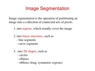
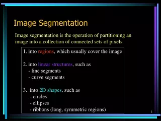
Introduction The purpose of image segmentation is to partition an image into meaningful regions with respect to a particular application The segmentation is based on measurements taken from the image and might be greylevel, colour, texture, depth or motion
Image Segmentation • Segmentation divides an image into its constituent regions or objects. • Segmentation of non trivial images is one of the difficult task in image processing. Still under research. • Segmentation accuracy determines the eventual success or failure of computerized analysis procedure.
Segmentation Algorithms • Segmentation algorithms are based on one of two basic properties of intensity values discontinuity and similarity. • First category is to partition an image based on abrupt changes in intensity, such as edges in an image. • Second category are based on partitioning an image into regions that are similar according to a predefined criteria. Histogram thresholding approach falls under this category.
Domain spaces • spatial domain (row-column (rc) space) • histogram spaces • color space • other complex feature space
image segmentation • Applications of image segmentation include • Identifying objects in a scene for object-based measurements such as size and shape • Identifying objects in a moving scene for object-based video compression (MPEG4) • Identifying objects which are at different distances from a sensor using depth measurements from a laser range finder enabling path planning for a mobile robots
Example 1 • Segmentation based on greyscale • Very simple ‘model’ of greyscale leads to inaccuracies in object labelling
Example 2 • Segmentation based on texture • Enables object surfaces with varying patterns of grey to be segmented
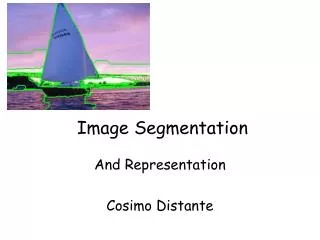
Example 3 • Segmentation based on motion • The main difficulty of motion segmentation is that an intermediate step is required to (either implicitly or explicitly) estimate an optical flow field • The segmentation must be based on this estimate and not, in general, the true flow
Example 4 • Segmentation based on depth • This example shows a range image, obtained with a laser range finder • A segmentation based on the range (the object distance from the sensor) is useful in guiding mobile robots
Introduction to image segmentation Range image Original image Segmented image
Histograms • Histogram are constructed by splitting the range of the data into equal-sized bins (called classes). Then for each bin, the number of points from the data set that fall into each bin are counted. • Vertical axis: Frequency (i.e., pixel counts for each bin) • Horizontal axis: Response variable • In image histograms the pixels form the horizontal axis
Thresholding - Foundation • Suppose that the gray-level histogram corresponds to an image f(x,y) composed of dark objects on the light background, in such a way that object and background pixels have gray levels grouped into two dominant modes. One obvious way to extract the objects from the background is to select a threshold ‘T’ that separates these modes. • Then any point (x,y) for which f(x,y) < T is called an object point, otherwise, the point is called a background point.
Gray Scale Image - bimodal Image of a Finger Print with light background
Segmented Image Image after Segmentation
Bimodal Histogram • If two dominant modes characterize the image histogram, it is called a bimodal histogram. Only one threshold is enough for partitioning the image. • If for example an image is composed of two types of dark objects on a light background, three or more dominant modes characterize the image histogram.
Multimodal Histogram • In such a case the histogram has to be partitioned by multiple thresholds. • Multilevel thresholding classifies a point (x,y) as belonging to one object class if T1 < (x,y) <= T2, to the other object class if f(x,y) > T2 and to the background if f(x,y) <= T1.
Thresholding Bimodal Histogram • Basic Global Thresholding: 1)Select an initial estimate for T 2)Segment the image using T. This will produce two groups of pixels. G1 consisting of all pixels with gray level values >T and G2 consisting of pixels with values <=T. 3)Compute the average gray level values mean1 and mean2 for the pixels in regions G1 and G2. 4)Compute a new threshold value T=(1/2)(mean1 +mean2) 5)Repeat steps 2 through 4 until difference in T in successive iterations is smaller than a predefined parameter T0. • Basic Adaptive Thresholding: Images having uneven illumination makes it difficult to segment using histogram, this approach is to divide the original image into sub images and use the above said thresholding process to each of the sub images.
Thresholding multimodal histograms • A method based on Discrete Curve Evolution is to find thresholds in the histogram. • The histogram is treated as a polylineand is simplified until a few vertices remain. • Thresholds are determined by vertices that are local minima.
Discrete Curve Evolution (DCE) It yields a sequence: P=P0, ..., Pm Pi+1 is obtained from Pi by deleting the vertices of Pi that have minimal relevance measure K(v, Pi) = |d(u,v)+d(v,w)-d(u,w)| v v > w w u u
Thresholding – Colour Images • In colour images each pixel is characterized by three RGB values. • Here we construct a 3D histogram, and the basic procedure is analogous to the method used for one variable. • Histograms plotted for each of the colour values and threshold points are found.
Displaying objects in the Segmented Image • The objects can be distinguished by assigning an arbitrary pixel value or average pixel value to the regions separated by thresholds.
Experiments by Venugual Rajagupal • Type of images used: 1) Two Gray scale image having bimodal histogram structure. 2) Gray scale image having multi-modal histogram structure. 3) Colour image having bimodal histogram structure.
Gray Scale Image - bimodal Image of rice with black background
Segmented Image Image after segmentation Image histogram of rice
Gray Scale Image - Multimodal Original Image of lena
Multimodal Histogram Histogram of lena
Segmented Image Image after segmentation – we get a outline of her face, hat, shadow etc
Colour Image - bimodal Colour Image having a bimodal histogram
Histogram Histograms for the three colour spaces
Segmented Image Segmented image – giving us the outline of her face, hand etc
Clustering in Color Space Each image point is mapped to a point in a color space, e.g.: Color(i, j) = (R (i, j), G(i, j), B(i, j)) The points in the color space are grouped to clusters. The clusters are then mapped back to regions in the image.
Results 1 Original pictures segmented pictures Mnp: 30, percent 0.05, cluster number 4 Mnp : 20, percent 0.05, cluster number 7
K-means clustering as before: vectors can contain color+texture CSE 803 Fall 2008 Stockman
K-means CSE 803 Fall 2008 Stockman
Segments formed by K-means CSE 803 Fall 2008 Stockman
Segmentation via region-growing (aggregation) Pixels, or patches, at the lowest level are combined when similar in a hierarchical fashion CSE 803 Fall 2008 Stockman
Decision: combine neighbors? Neighboring pixel or region CSE 803 Fall 2008 Stockman
Aggregation decision CSE 803 Fall 2008 Stockman
Representation of regions CSE 803 Fall 2008 Stockman
Chain codes for boundaries CSE 803 Fall 2008 Stockman
Quad trees divide into quadrants M=mixed; E=empty; F=full CSE 803 Fall 2008 Stockman
Can segment 3D images also • Oct trees subdivide into 8 octants • Same coding: M, E, F used • Software available for doing 3D image processing and differential equations using octree representation. • Can achieve large compression factor. CSE 803 Fall 2008 Stockman
Conclusion Segmentation algorithms generally are based on one of 2 basis properties of intensity values discontinuity : to partition an image based on sharp changes in intensity (such as edges) similarity : to partition an image into regions that are similar according to a set of predefined criteria.