Download
1 / 33
350 likes | 469 Vues
Explore tree and graph algorithms with real-world applications and algorithmic elegance. Learn about Google's Page Rank, Directed Acyclic Word Graph, heap data structure, and the power of algorithmic thinking.

E N D
More Algorithmsfor Trees and Graphs Eric Roberts CS 106B March 11, 2013
Outline for Today • The plan for today is to walk through some of my favorite tree and graph algorithms, partly to demystify the many real-world applications that make use of those algorithms and partly to emphasize the elegance and power of algorithmic thinking. • These algorithms include: • Google’s Page Rank algorithm for searching the web • The Directed Acyclic Word Graph format used in Lexicon • The heap data structure used to create efficient priority queues
Google The big innovation of the late 1990s is the development of search engines, which began with Alta Vista at DEC’s Western Research Lab and reaching its modern pinnacle with Google, which was founded by Stanford graduate students Larry Page and Sergey Brin in 1998. Larry Page and Sergey Brin
Page Rank The heart of the Google search engine is the page rank algorithm, which was described in a 1999 by Larry Page, Sergey Brin, Rajeev Motwani, and Terry Winograd. The PageRank Citation Ranking: Bringing Order to the Web January 29, 1998 Abstract The importance of a Webpage is an inherently subjective matter, which depends on the reader’s interests, knowledge and attitudes. But there is still much that can be said objectively about the relative importance of Web pages. This paper describes PageRank, a method for rating Web pages objectively and mechanically, effectively measuring the human interest and attention devoted to them. We compare PageRank to an idealized random Websurfer. We show how to efficiently compute PageRank for large numbers of pages. And,we show how to apply PageRank to search and to user navigation.
Page Rank Algorithm The page rank algorithm gives each page a rating of its importance, which is a recursively defined measure whereby a page becomes important if other important pages link to it. One way to think about page rank is to imagine a random surfer on the web, following links from page to page. The page rank of any page is roughly the probability that the random surfer will land on a particular page. Since more links go to the important pages, the surfer is more likely to end up there.
A simple example of a Markov process is illustrated by this table, which shows the likelihood of a particular weather pattern for tomorrow given the weather for today. What, then, is the likely weather two days from now, given that you know what the weather looks like today? What if you then repeat the process for ten days? If today is 0.85 0.10 0.05 0.81 0.77 0.14 0.13 0.06 0.07 0.60 0.25 0.15 0.72 0.77 0.18 0.14 0.10 0.07 0.40 0.40 0.20 0.66 0.77 0.14 0.22 0.12 0.07 Markov Processes Google’s random surfer is an example of a Markov process, in which a system moves from state to state, based on probability information that shows the likelihood of moving from each state to every other possible state. That far out, it doesn’t matter what today’s weather is. The day after tomorrow will be Ten days from now will be Tomorrow will be
1. Start with a set of pages. The Page Rank Algorithm A B D E C
2. Crawl the web to determine the link structure. The Page Rank Algorithm A B D E C
3. Assign each page an initial rank of 1 / N. The Page Rank Algorithm A B 0.2 0.2 D 0.2 E C 0.2 0.2
4. Successively update the rank of each page by adding up the weight of every page that links to it divided by the number of links emanating from the referring page. D 0.2 E C 0.2 0.2 PR(C) PR(D) 0.2 0.2 PR(E) = 0.17 + = + 3 2 3 2 The Page Rank Algorithm • In the current example, page E has two incoming links, one from page C and one from page D. • Page C contributes 1/3 of its current page rank to page E because E is one of three links from page C. Similarly, pageDoffers 1/2 of its rank to E. • The new page rank for E is
5. If a page (such as E in the current example) has no outward links, redistribute its rank equally among the other pages in the graph. D 0.2 E C 0.2 0.2 The Page Rank Algorithm • In this graph, 1/4 of E’s page rank is distributed to pages A, B, C, and D. • The idea behind this model is that users will keep searching if they reach a dead end.
7. Apply this redistribution to every page in the graph. The Page Rank Algorithm A B 0.28 0.15 D 0.18 E C 0.17 0.22
8. Repeat this process until the page ranks stabilize. The Page Rank Algorithm A B 0.26 0.17 D 0.17 E C 0.16 0.23
9. In practice, the Page Rank algorithm adds a damping factor at each stage to model the fact that users stop searching. The Page Rank Algorithm A B 0.25 0.17 D 0.18 E C 0.17 0.22
Directed Acyclic Word Graphs • The Lexicon class provides a highly time- and space-efficient representation of a word list. • The data representation used in the Lexicon class is called a Directed Acyclic Word Graph or DAWG, which was first described in a 1988 paper by Appel and Jacobson. • The DAWG structure is based on a much older data structure called a trie, developed by Ed Fredkin in 1960. (The trie data structure is described in the text on page 490.)
The Trie Data Structure • The trie representation of a word list uses a tree in which each arc is labeled with a letter of the alphabet. In a trie, the words themselves are represented implicitly as paths to a node.
Going to the DAWGs • The new insight in the DAWG is that you can combine nodes that represent common endings. • As the authors note, “this minimization produces an amazing savings in space; the number of nodes is reduced from 117,150 to 19,853.”
The Heap Algorithm • If you implement them in the obvious way using either arrays or linked lists, priority queues require O(N) time. Because priority queues are essential to both Dijkstra’s and Kruskal’s algorithms, making them efficient improves performance. • The standard algorithm for implementing priority queues uses a data structure called a heap, which makes it possible to implement priority queue operations in O(logN) time. • A heap is a binary tree with three additional properties: • The tree is complete, which means that it is not only completely balanced but that each level of the tree is filled as far to the left as possible. • The root node of the tree has higher priority than the root of either of its subtrees. • Every subtree is also a heap.
Exercise: Tracing the Heap Algorithm Insert in order: 17 93 20 42 68 11 17
Exercise: Tracing the Heap Algorithm Insert in order: 17 93 20 42 68 11 17 93
Exercise: Tracing the Heap Algorithm Insert in order: 17 93 20 42 68 11 17 20 93
Exercise: Tracing the Heap Algorithm Insert in order: 17 93 20 42 68 11 17 20 93 42
Exercise: Tracing the Heap Algorithm Insert in order: 17 93 20 42 68 11 17 20 93 42
Exercise: Tracing the Heap Algorithm Insert in order: 17 93 20 42 68 11 17 20 42 68 93
Exercise: Tracing the Heap Algorithm Insert in order: 17 93 20 42 68 11 17 20 42 11 68 93
Exercise: Tracing the Heap Algorithm Insert in order: 17 93 20 42 68 11 17 20 42 11 68 93
Exercise: Tracing the Heap Algorithm Insert in order: 17 93 20 42 68 11 17 11 42 20 68 93
Exercise: Tracing the Heap Algorithm Insert in order: 17 93 20 42 68 11 Dequeue the top priority element 11 17 42 20 68 93
Exercise: Tracing the Heap Algorithm Insert in order: 17 93 20 42 68 11 Dequeue the top priority element 11 20 17 42 68 93
Exercise: Tracing the Heap Algorithm Insert in order: 17 93 20 42 68 11 Dequeue 11