SamplePoint Tutorial SamplePoint is a tool that facilitates point-sampling of digital images.

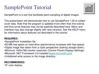
1. SamplePoint Tutorial • SamplePoint is a tool that facilitates point-sampling of digital images. • This presentation will demonstrate how to use SamplePoint 1.25 to collect cover data. Note that the program is updated more often than this tutorial, and thus some features may not be explicitly described here. Menu and interface may also change slightly with new versions. See the HELP menu for information about features not described in the tutorial. • REQUIRED: • SamplePoint Installation file • 50 MB free space on hard drive (performance increases with free space) • Digital image files taken from a nadir perspective (looking straight down). • Minimum 1024x768 monitor resolution (Control Panel>Display>Settings) • Microsoft .NET Framework 2.0 installed (www.microsoft.com) • Unfettered write access to the image directory • RECOMMENDED: • 19” color display

2. Obtain the SamplePoint installation file and double-click to begin installation.Follow the on-screen directions. The following files will be loaded onto your PC into the specified directory: SamplePoint.exe SamplePointTutorial.pps (this file) SamplePointHelp.pdf (requires Acrobat Reader) SPDB.xls Nadir Sample Image : dubois_41.bmp The Nadir Sample Image is the same images used in this tutorial. It was acquired from 2m above ground level using an aluminum camera stand and an Olympus E20 digital SLR camera, and covers approx. 1m x 1m with a ground sample distance of approx. 0.9 mm.

3. Use a camera stand to acquire nadir images using a digital camera. 1 mm GSD

4. Use a light airplane to acquire large-scale nadir images 2 mm GSD

5. Use an airplane or helicopter to acquire small scale nadir images 1 m GSD

6. Save digital images to your hard drive in TIFF or BMP form. JPEG is a lossy-format and is therefore not recommended for point sampling. Images MUST be nadir!

7. Open SamplePoint by double-clicking on SamplePoint.exe. If you encounter trouble, please reference “SamplePointHelp.PDF” in the program directory.

8. Click Options>Database Wizard. Provide a name for the database, then click Create/Populate Database.

9. Navigate to the folder containing the images you wish to classify. Click on the first image, then click on the last image while holding the Shift key to select all images. Ctrl+click selects individual images. No more than 200 images may be added to the database using the Wizard. To add more than 200 images, see the Help file on manual database editing. Finally, click Open.

10. Images may only be selected from one folder. All images must be selected at once (you cannot populate the database twice using the wizard). After images have been selected, click Done. The database is saved to, and must remain in, the folder containing the analysis images.

11. Click Options>Select Database and navigate to the image folder and select the *.xls file. Click Open.

12. A Pop-up box will confirm the number of images in the database. Click OK if this is correct.

13. The first image listed in the database (Image Key 1) will appear in the screen at full-view. To begin classification using default settings of 100 systematic points and 8 default classes, click Begin. Shows the image file and database Key

14. You are taken to point 1 in the upper left corner of the grid. Zoom in by pressing the ↑ key on your keyboard, zoom out by pressing ↓ key, or zoom by typing a value in the Zoom box and pressing Refresh.

15. Zoomed in to 28X.

16. Zoomed out to 4X. Note that the point is no longer centered as you zoom further out and are on the edge of the image.

17. You should be able to distinguish individual pixels. The goal is to classify the single pixel in the center of the crosshairs. Zoom out if needed to gain perspective.

18. Classify by clicking on the button below the image which describes the point. In this case, Soil. The button will flash red, then you will be taken to point 2. The classification is saved to the database.

19. Note that the point number is displayed in the lower left corner. The zoom setting stays the same from point to point unless you change it. Classify point 2: It is close to a piece of litter, but the center pixel is in fact soil. Zoom in if you are unsure.

20. Now you’re on point 3. If you feel you made a mistake on point 2, you can click the Back button to go back and reclassify point 2. If you want to start over at point 1 or go back 10 points at once, type in the target point number in the lower left corner “point” box, then click the RST (reset) button. Point X,Y location is indefinitely constant for each image unless you alter the grid size.

21. A notification pop-up appears when the final point for each image is classified. Click OK, then click the Next Image button to continue to the Image Key 2.

22. The next image will appear at full size. Note the Key now reads 2. Click Begin to start classification.

23. At no point do you need to save anything. All saving of classified points is done automatically and instantly by SamplePoint. You can Exit at any time, even in the middle of an image, without losing any data. To restart at a different time on a particular image, select the database, then click Options>Go To Image, and type in the KEY of the image you want to start with. Click OK and the image will load.

24. The Unknown button is useful for places like shadow, where the actual groundcover cannot be discerned.

25. A notification appears when the data set is complete. Click OK.

26. Click Options>Create Statistics Files. This generates two comma-delimited text files with a summary of the results. You can create these files at any time during the classification process, instead of waiting until all images are classified. These files are saved to the image folder.

27. After the Statistics Files are created, look in the image folder. You’ll see the database Excel file (DUBOIS2005.XLS), the Custom Button file (GreenBrownClasses.Btn) and two text files beginning with the database name, and ending with either .rgb or .txt. The .txt file is the cover summary that can be opened in either Notepad or Excel. The .rgb file is simply a comma-delimited list of each classification with respective red, green and blue pixel values. This is sometimes useful to compare pixel color distribution among different classes. It too can be opened in either Notepad or Excel.

28. If you Exit SamplePoint, you can examine the database using Excel. It shows the Key, Image file, Gridsize and classification of each point. The numbers beside the classification are the RGB values for the classified pixel. Custom button information is also stored in the database in columns HU-HW. You cannot open the database in SamplePoint if it is open in Excel on your PC, and vice-versa. You can add image files to the database manually using Excel by typing in additional keys and filenames or pasting them from a list. Filenames are case sensitive.

29. To open the summary file, Click File>Open, navigate to the image folder, then select Files of Type: All Files (*.*). Open the *_Summary.txt file. To import the text file, choose file type DELIMITED, and click OK. Then specify that the COMMA is the delimiter, click OK, then FINISH.

30. This is the Summary file displayed in Excel. It shows the % cover for each image by cover type. For each cover class, the first column shows the actual number of hits, and the second column shows the percent of hits in the image. With 100 points, %Grass=Grass and %Forb=Forb, etc., but this is not true if any number other than 100 points are classified.

31. The RGB file is opened and examined in the same way as the Summary file. This file allows easy mathematical summary and analysis of the class color characteristics.

32. OPTIONS • Defining custom classes • Changing the number of classification points • Random classification points

33. To create up to 30 custom classes, click Options>Custom Buttons>Create Custom Button Files. Define the button labels with titles of 6-7 characters each. Click Save when complete.

34. Navigate to the Image folder, name the button class file, then click Save.

35. To activate the custom buttons, click Options>Custom Buttons>Load Custom Button File. Select the file you just created, or some other *.btn file. Click Open. You must have a database loaded before you can load a custom button file.

36. The custom classes are now ready to use. The data saved to the database will be saved using these classes. The custom buttons must be in place prior to classification, with one exception: A class can be added to the end of a custom button file at any time with no adverse effect. Just follow the same steps as above and overwrite the old button file.

37. To change the number of classification points, click Options>Select Grid Size> and select the desired number of points. All points are systematically placed with equal points in rows and columns. The selected grid is used for all subsequent images unless you change it, or exit the software.

38. For random points, click Options>Select Grid Size>Random Points. A pop-up box appears in which you must select the precise number of classification points you want from 1 to 200. Since point distribution is random each time, you cannot return to these points at a later date, as you can with the systematic point grid. Consider carefully if this is an option you will need.

39. APPLICATIONS The previous example utilized images taken with the camera positioned 2m above ground level (AGL) using a camera stand. Aerial images are also easily analyzed using SamplePoint.

40. This aerial image was acquired 100m AGL from a light airplane. SamplePoint operates in the same way regardless of the image type. Note the new custom buttons specific to this project.

41. This image was acquired from 3000m AGL. Landscape-scale cover types, such as riparian zone, conifer forest, sagebrush steppe, etc., can be obtained using SamplePoint.

42. APPLICATIONS Previous examples demonstrates how to obtain cover measurements over an entire image, but cover measurements can also be made within a specific area of the image. For example, a user wants to measure the % willow cover within the riparian area, and the % sagebrush cover in the surrounding upland area. This can be done using 4 customized buttons: Willow, Sagebrush, Riparian-not willow (Rip-nw) and Upland-not Sagebrush (Up-ns)

43. The custom buttons are created and loaded,and a database is created with a single aerial image (≈ 2cm GSD).

44. Points falling in water are here classified as “Riparian-not willow” but it would be a simple change to add a separate water class for those points.

45. Classification results: Sagebrush = 6% Upland Non-sagebrush = 39% Willow = 15% Riparian Non-willow = 40% An implicit assumption is that sagebrush are found only in upland areas, and willows are found only in riparian areas. If this assumption is true, then any point classified as willow is inherently classified as riparian. Thus, willow cover in the riparian area is calculated as: Willow / (Willow + Riparian Non-Willow) = 15 / (15 + 40) = 27% And, sagebrush cover in surrounding upland area is calculated as: Sagebrush / (Sagebrush + Upland Non-sagebrush) = 6 / (6 + 39) = 13% Conclusion of this classification: Willow cover in the riparian area is 27%, and Sagebrush cover in the surrounding upland area is 13%.

46. APPLICATIONS Because systematic classification points are assigned based on image size, and are always located in the same X,Y position for images of equal size, SamplePoint provides a simple way to perform accuracy assessments on image classification by software like Erdas Imagine or VegMeasurement.

47. Export the processed image from VegMeasure or Imagine as a TIF or BMP, and run both the original and processed images through SamplePoint. In this example, a processed image from VegMeasurement was used. Since point 1 will occupy the same X,Y location on both images, classification accuracy can be determined by comparing the known to classified for a number of points over a number of images. For example, point 1 in the original image is classified as bare ground. Point 1 in the classified image is white, so point 1 was correctly classified. To perform the assessment, the first step is to classify all points into the classes of interest, though you cannot change buttons mid-assessment. In this example, white color is classified as bare ground, black is classified as other. REMEMBER: You must use systematic point distribution for this operation.

48. The second step takes place in Excel. Sort the data from the database into two columns, where original images line up with processed images precisely. For example, point 56 of original image 28 lines up with point 56 of processed image 28. Sort both columns in ascending order. For a binary classification, this will lump the data into 4 groups: Other – Other (Correct classification) Bare – Bare (Correct classificaiton) Other - Bare (Omission error) Bare – Other (Commission error) Overall accuracy is calculated as: Correct / (Correct + Incorrect) The use of an error matrix will facilitate the calculation of user’s and producer’s accuracy rates (Congalton 1991). This technique allows, by default, an assessment of user classification accuracy. If bare ground is always white in the processed image, then any point with black RGB values that is classified as bare ground is an error, and vice versa. This yields the user error rate, as opposed to the software error rate. Congalton, RG. 1991. A review of assessing the accuracy of classification of remotely sensed data. Remote Sens. Environ. 37:35-46.

49. A simple error matrix set up with original image classification data in columns, and processed-image classification data in rows. For example, a total of 494 points were classified as Bare Ground in the original images, but only 194 points were so classified by the automated analysis. Overall Accuracy = (60 + 1372)/2000 = 71.6% This is often a misleading statistic if what you’re really interested in is a small class, such as bare ground. Measures of accuracy that ignore other classes are more useful. Bare Ground: Producer’s Accuracy: Probability that a point of known cover type is correctly classified by the software. 60/494 = 12.1% User’s Accuracy: Probability that a point classification made by the software is correct. 60/194 = 30.9%

50. The SamplePoint concept was developed by the USDA Agricultural Research Service, Rangeland Resources Research Unit in Cheyenne, Wyoming, funded in part by the USDI Bureau of Land Management Wyoming State Office. Software code was written by Robert Berryman. Installation file was generated using Nullsoft Install System v 2.11. For user information not covered in this tutorial, click Help>Contents to open the PDF Help File. This Tutorial is current as of Sept 4, 2007. For technical assistance, contact Terry Booth or Sam Cox at 307-772-2433. USDA ARS RRRU 8404 Hildreth Rd Cheyenne, WY 82009