Download
1 / 28
280 likes | 470 Vues
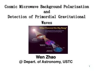
CMB Polarization Generated by Primordial Gravitational Waves - Analytical Solutions. Alexander Polnarev Queen Mary, University of London MG12, Paris, 13 July 2009. The Beginning of Polarization Theory in Cosmology

E N D
CMB Polarization Generated by Primordial Gravitational Waves - Analytical Solutions Alexander Polnarev Queen Mary, University of London MG12, Paris, 13 July 2009
The Beginning of Polarization Theory in Cosmology Originally proposed by Rees (1968) as an observational signature of an Anisotropic Universe [Caderni et al (1978), Basko, Polnarev (1979), Lubin et al (1979), Nanos et al (1979)] The polarization of the cosmic microwave background (CMB) was unobserved for 34 years
This presentation is using the results of the following papers: I. “The polarization of the Cosmic Microwave Background due to Primordial Gravitational Waves”, B.G.Keating, A.G.Polnarev, N.J.Miller and D.Baskaran. International Journal of Modern Physics A, Vol. 21, No. 12, pp. 2459-2479 (2006) II. “Imprints of Relic Gravitational Waves on Cosmic Microwave Background Radiation”, D.Baskaran, L.P.Grishchuk and A.G.Polnarev, Physical Review D 74, 083008 (2006)
At a given spatial position the CMB is characterized by: 1) its frequency spectrum: black body, with temperature ~ 2.728°K. 3) polarization of CMB. ~ 1 part in 106 2) angular anisotropy (i.e. variations in CMB intensity in different directions): ~ 1 part in 105 (excluding the dipole). Pictures taken from LAMBDA archive http://lambda.gsfc.nasa.gov/
Choosing a x,y coordinate frame in the plane orthogonal to the line of sight, these are related to possible quadratic time averages of the electromagnetic field: I is the total intensity of the radiation field Q and U quantify the direction and the magnitude of the linear polarization. V characterizes the degree of circular polarization At a given observation point, for a particular direction of observation the radiation field can be characterized by four Stokes parameters conventionally labeled as I,Q,U,V: In order to proceed let us firstly recap the main characteristics of the radiation field…
Physics of polarization creation due to the Thompson scattering of anisotropic radiation: The structure of the Thompson scattering is such that it requires a quadrupole component of anisotropy to produce linear polarization! (Animation taken from Wayne Hu homepage : http://background.uchicago.edu/~whu/) The metric perturbations directly couple only to anisotropies, i.e. they only directly create an unpolarized temperature anisotropy. Polarization is created by the Thompson scattering of this anisotropic radiation from free electrons!
Introducing a spherical coordinate system , as a function of the direction of observation on the sky, the four Stokes parameters form the components of the polarization tensor Pab : Two other invariant quantities characterizing the linear polarization can be constructed by covariant differentiation of the symmetric trace free part of the polarization tensor: Which is known as the E-mode of polarization, and is a scalar. Which is known as the B-mode of polarization, and is pseudoscalar. The components of the polarization tensor are not invariant under rotations, and transform through each other under a coordinate transformation. For this reason it is convenient to construct rotationally invariant quantities out of Pab Two of the obvious quantities are: which (as was mentioned before) characterizes the total intensity, and is a scalar under coordinate transformations. Which characterizes the degree of circular polarization, and behaves as a pseudoscalar under coordinate transformations
The most important thing is that the E mode is different from the B mode The mathematical formulae from the previous slide allow to separate the two types
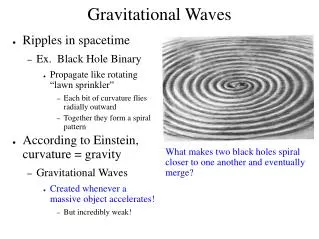
Gravitational Waves • Gravitational waves show a power spectrum with both the E and the B mode contributions • Gravitational waves’ contribution to the B-modes is a few tenths of a μK at l~100. • Gravitational waves probe the physics of inflation but will require a thorough understanding of the foregrounds and the secondary effects for their detection.
Where is a symbolic 3-vector, the components of which are expressible through the Stokes parameters Encodes the information on the scattering mechanism Couples the metric through covariant differentiation In the cosmological context (for z<<10^6), the dominant mechanism is the Thompson scattering! Where is the photon 4 momentum, is the direction of photon propagation, and is the photon frequency. Is the Chandrasekhar scattering matrix for Thompson scattering. is the Thompson scattering cross section. is the density of free electrons Thompson scattering and Equation of radiative transfer: Symbolically the radiative transfer equation has the form of Liouville equation in the photon phase space
Where the unperturbed part corresponds to an isotropic and homogeneous radiation field: (Corresponds to an overall redshift with cosmological expansion.) The first order equation (restricting only to the linear order) takes the form: Thompson scattering (where and ) metric perturbations The solution to the radiative transfer equation is sought in the form:
determines anisotropy while determines polarization. determines the (photon) frequency dependency of both anisotropy and polarization (the dependence is same for both)! The problem has simplified to solving for two functions and of two variables . (initially we had variables , 1+3+1+2=7 variables. ) Here is the angle between the angle of sight e and the wave vector n. And is the angle in the azimuthal plane (i.e. plane perpendicular to n). Due to the linear nature of the problem and in order to simplify the equations, we can Fourier (spatial) decompose the solution, and consider each individual Fourier mode separately For each individual Fourier mode, without the loss of generality the solution can be sought in the form (Basko&Polnarev1980):
The equations for and have the form of an integro-differential equation in two variables (Polnarev1985): (Thompson scattering term) (Density of free electrons) Anisotropy is generated by the variable g.w. field and by scattering! Polarization is generated by scattering of anisotropy where
The usual approach to the problem of solving these equations is to decompose and in over the variable terms of Legendre polynomials. The expected power spectra of anisotropy and polarization can then be expressed in terms of and . This procedure leads to an infinite system of coupled ordinary differential equations for each l ! The standard numerical codes like CMBFast and CAMB are based on solving an (appropriately cut) version of these equations!
Further introducing two functions Optical depth Visibility function Thus both (anisotropy) and (polarization) are expressible through a single unknown function ! A n alternative approach to the problem is to reduce above equations to a single integral equation. In order to do this let us first introduce two quantities which will play an important role in further considerations: The formal solution to equations for and is given by:
The equation for can be arrived at by substituting the above formal solution into the initial system for and . The result is a single Voltaire type integral equation in one variable: Where is the gravitational wave source term for polarization and the Kernels are given by:
Take an arbitrary Φ and calculate analytically the corresponding Φ0 Compare the numerically obtained Φwith the original Φ! Solve the integral equation numerically with this Φ0. Find numerical solution Φ for a given Φ0 Insert this Φ back into the integral equation and calculate Φ0. Compare the new Φ0 with the original Φ0! Precision control The integral equation for the function Φ allows for a very simple precision control. A very simple algorithm lets us control the precision of the numerical evaluation: OR
Advantages of the integral equation: • The integral equation allows to recast the problem in a mathematically closed form. • It is a single equation instead of an infinite system of coupled differential equations. • Computationally it is quicker to solve. Precision control is simpler. • Allows for simpler analytical manipulations, and yields a solution in the form of an infinite series. • Allows for an easier understanding of physics (my subjective impression!).
Polarization window function Polarization window function for secondary ionization The solution of the integral equation depends crucially on the Polarization window function Q (η)=q (η) exp(-τ(η)) .
The main thing to keep in mind is that in the lowest approximation: Anisotropy is proportional to g.w. wave amplitude at recombination. While polarization is proportional to the amplitude of the derivative at recombination. where With each term expressible through a recursive relationship: Where Kernels are dependent only on the recombination history: The integral equation can be either solved numerically, or the solution can be presented in the form of a series in over (which for wavelengths of our interest l<1000 is a small number).
(Solid line shows the exact numerical solution, while the dashed line shows the zeroth order analytical approximation.) The solution is localized around the visibility function (around the epoch of recombination). Physically this is a consequence of the fact that: on the one hand due to the enormous optical depth before recombination we cannot see the polarization generated much before recombination on the other hand polarization generation requires free electrons, which are absent after the recombination is complete. The solution to the integral equation for various wavenumbers:
Low frequency approximation: High frequency approximation:
Let us introduce the following elementary integral operators
Low frequency approximation In limiting case when k0 We have the following expansion for the operator :
High frequency approximation In opposite limiting case when k We have the following asymptotic expansion for the operator : where C plays the role of constant of integration over k and can be obtained from asymptotic k .
Summary and Conclusions: We have conducted a semi-analytical study of anisotropy and polarization of CMB due to primordial gravitational waves. Mathematically the problem has been formulated in terms of a single Voltairre type integral equation (instead of a infinite system of coupled differential equations). This method allows for a simpler numerical evaluation, as well as a clearer understanding of the underlying physics. The main features in the anisotropy and polarization spectra due to primordial g.w. have been understood and explained. With the currently running and future planned CMB experiments there seems to be a good chance to observe primordial g.w.s . CMB promises to be our clearest window to observe primordial g.w..