Understanding Sampling Distributions: Key Concepts, Estimation, and Significance Testing

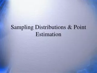
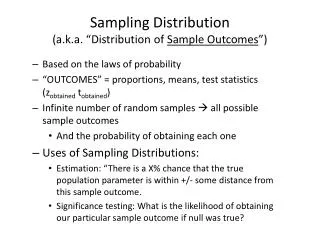
1. Sampling Distribution(a.k.a. “Distribution of Sample Outcomes”) • Based on the laws of probability • “OUTCOMES” = proportions, means, test statistics (zobtainedtobtained) • Infinite number of random samples  all possible sample outcomes • And the probability of obtaining each one • Uses of Sampling Distributions: • Estimation: “There is a X% chance that the true population parameter is within +/- some distance from this sample outcome. • Significance testing: What is the likelihood of obtaining our particular sample outcome if null was true?

2. Estimation Review • Point Estimate • Proportion or Mean • Confidence interval • Confidence level (1-alpha) • Dictates how many standard errors to go out on the sampling distribution • Normal (z-score) distribution for mean and proportion • What is one standard error “worth” • Formulas for proportion, mean

3. Significance Testing • State a Null Hypothesis • Calculate the odds of obtaining your sample finding if that null hypothesis is correct • Compare this to the odds that you set ahead of time (e.g., alpha) • If odds are less than alpha, reject the null in favor of the research hypothesis • The sample finding would be so rare if the null is true that it makes more sense to reject the null hypothesis

4. If we did a gazillion samples, UNDER NULL, and plotted mean differences…sampling distribution of difference between means N = 150 X=4.0 X-μ 4 - 4.5=0. μ = 4.5 (N=50) X-μ 4.7 - 4.5=0.2 CHILDREN’S AGE IN YEARS N = 150 X=4.7

5. You would get a sampling distribution • Sampling distribution of the difference between means • If large enough sample (N>100), it would be normal • Use “z-scores” or “obtained” and “critical” z values • If smaller samples, no longer perfectly normal • Use “t-scores” • t distribution changes with sample size • CHART for critical t values

6. Significance the old fashioned way • Find the “critical value” of the test statistic for your sample outcome • Z tests always have the same critical values for given alpha values (e.g., .05 alpha  +/- 1.96) • Use if N >100 • t values change with sample size • Use if N < 100 • As N reaches 100, t and z values become almost identical • Compare the critical value with the obtained value  Are the odds of this sample outcome less than 5% (or 1% if alpha = .01)?

7. Critical Values/Region for the z test( = .05)

8. Directionality • Research hypothesis must be directional • Predict how the IV will relate to the DV • Males are more likely than females to… • Southern states should have lower scores…

9. Non-Directional & Directional Hypotheses • Nondirectional • Ho: there is no effect: (X = µ) • H1: there IS an effect: (X ≠ µ) • APPLY 2-TAILED TEST • 2.5% chance of error in each tail • Directional • H1: sample mean is larger than population mean (X > µ) • Ho x ≤ µ • APPLY 1-TAILED TEST • 5% chance of error in one tail -1.96 1.96 1.65

10. Example: Single sample means, smaller N A random sample of 16 UMD students completed an IQ test. They scored an average of 104, with a standard deviation of 9. The IQ test has a national average of 100. IS the UMD students average different form the national average?

11. Answer #1 Conceptually • Under the null hypothesis (no difference between means), there is more than a 5% chance of obtaining a mean difference this large. Sampling distribution for one sample t-test (a hypothetical plot of an infinite number of mean differences, assuming null was correct) t (obtained) = 1.72 Critical Region Critical Region -2.131 (t-crit, df=15) 2.131(t-crit, df=15)