Unsupervised Learning and Clustering

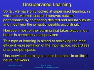
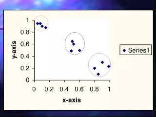
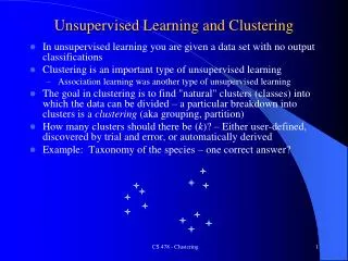
1. Unsupervised Learning and Clustering • In unsupervised learning you are given a data set with no output classifications • Clustering is an important type of unsupervised learning • Association learning was another type of unsupervised learning • The goal in clustering is to find "natural" clusters (classes) into which the data can be divided – a particular breakdown into clusters is a clustering (aka grouping, partition) • How many clusters should there be (k)? – Either user-defined, discovered by trial and error, or automatically derived • Example: Taxonomy of the species – one correct answer? CS 478 - Clustering

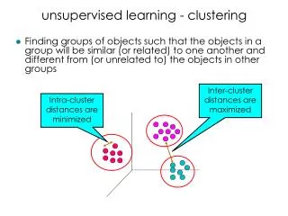
2. Clustering • How do we decide which instances should be in which cluster? • Typically put data which is "similar" into the same cluster • Similarity is measured with some distance metric • Also try to maximize a between-class dissimilarity • Seek balance of within-class similarity and between-class difference • Similarity Metrics • Euclidean Distance most common for real valued instances • Can use (1,0) distance for nominal and unknowns like with k-NN • Important to normalize the input data CS 478 - Clustering

3. Outlier Handling • Outliers • noise, or • correct, but unusual data • Approaches to handle them • become their own cluster • Problematic, e.g. when k is pre-defined (How about k = 2 above) • If k=3 above then it could be its own cluster, rarely used, but at least it doesn't mess up the other clusters • Could remove clusters with 1 or few elements as a post-process step • absorb into the closest cluster • Can significantly adjust cluster radius, and cause it to absorb other close clusters, etc. – See above case • Remove with pre-processing step • Detection non-trivial – when is it really an outlier? CS 478 - Clustering

4. Distances Between Clusters • Easy to measure distance between instances (elements, points), but how about the distance of an instance to another cluster or the distance between 2 clusters • Can represent a cluster with • Centroid – cluster mean • Then just measure distance to the centroid • Medoid – an actual instance which is most typical of the cluster • Other common distances between two Clusters A and B • Single link – Smallest distance between any 2 points in A and B • Complete link – Largest distance between any 2 points in A and B • Average link – Average distance between points in A and points in B CS 478 - Clustering

5. Partitional and Hierarchical Clustering • Two most common high level approaches • Hierarchical clustering is broken into two approaches • Agglomerative: Each instance is initially its own cluster. Most similar instance/clusters are then progressively combined until all instances are in one cluster. Each level of the hierarchy is a different set/grouping of clusters. • Divisive: Start with all instances as one cluster and progressively divide until all instances are their own cluster. You can then decide what level of granularity you want to output. • With partitional clustering the algorithm creates one clustering, typically by minimizing some objective function • Note that you could run the partitional algorithm again in a recursive fashion on any or all of the new clusters if you want to build a hierarchy CS 478 - Clustering

6. Hierarchical Agglomerative Clustering (HAC) • Input is an n × n adjacency matrix giving the distance between each pair of instances • Initialize each instance to be its own cluster • Repeat until there is just one cluster containing all instances • Merge the two "closest" remaining clusters into one cluster • HAC algorithms vary based on: • "Closeness definition", single, complete, or average link common • Which clusters to merge if there are distance ties • Just do one merge at each iteration, or do all merges that have a similarity value within a threshold which increases at each iteration CS 478 - Clustering

7. Dendrogram Representation A B C E D • Standard HAC • Input is an adjacency matrix • output can be a dendrogram which visually shows clusters and merge distance CS 478 - Clustering

8. Which cluster level to choose? • Depends on goals • May know beforehand how many clusters you want - or at least a range (e.g. 2-10) • Could analyze the dendrogram and data after the full clustering to decide which subclustering level is most appropriate for the task at hand • Could use automated cluster validity metrics to help • Could do stopping criteria during clustering CS 478 - Clustering

9. Cluster Validity Metrics - Compactness • One good goal is compactness – members of a cluster are all similar and close together • One measure of compactness of a cluster is the SSE of the cluster instances compared to the cluster centroid • where c is the centroid of a cluster C, made up of instances Xc. Lower is better. • Thus, the overall compactness of a particular clustering is just the sum of the compactness of the individual clusters • Gives us a numeric way to compare different clusterings by seeking clusterings which minimize the compactness metric • However, for this metric, what clustering is always best? CS 478 - Clustering

10. Cluster Validity Metrics - Separability • Another good goal is separability – members of one cluster are sufficiently different from members of another cluster (cluster dissimilarity) • One measure of the separability of two clusters is their squared distance. The bigger the distance the better. • distij = (ci - cj)2 where ci and cj are two cluster centroids • For a clustering which cluster distances should we compare? CS 478 - Clustering

11. Cluster Validity Metrics - Separability • Another good goal is separability – members of one cluster are sufficiently different from members of another cluster (cluster dissimilarity) • One measure of the separability of two clusters is their squared distance. The bigger the distance the better. • distij = (ci - cj)2 where ci and cj are two cluster centroids • For a clustering which cluster distances should we compare? • For each cluster we add in the distance to its closest neighbor cluster • We would like to find clusterings where separability is maximized • However, separability is usually maximized when there are are very few clusters • squared distance amplifies larger distances

12. Davies-Bouldin Index • One answer is to combine both compactness and separability into one metric seeking a balance • One example is the Davies-Bouldin index which scores a specific clustering • Define • where |Xc| is the number of elements in the cluster represented by the centroid c, and|C| is the total number of clusters in the clustering • Want small scatter – small compactness with many cluster members • For each cluster i, ri is maximized for a close neighbor cluster with high scatter (measures worse case close neighbor, hope these are low as possible) • Total cluster score ris just the sum of ri. Lower r better. • ris small when cluster distances are greater and scatter values are smaller • Davies-Bouldin score r finds a balance of separability (distance) being large and compactness (scatter) being small • We don’t actually minimize r over all possible clusterings, as that is exponential. But we can calculate rvalues to compare whichever clusterings our current algorithm explores. • There are other cluster metrics out there • These metrics are rough guidelines and must be "taken with a grain of salt" CS 478 - Clustering

13. HAC Summary • Complexity – Relatively expensive algorithm • n2 space for the adjacency matrix • mn2 time for the execution where m is the number of algorithm iterations, since we have to compute new distances at each iteration. m is usually ≈ n making the total time n3 • All k (≈ n)clusterings returned in one run. No restart for different k values • Single link – (nearest neighbor) can lead to long chained clusters where some points are quite far from each other • Complete link – (farthest neighbor) finds more compact clusters • Average link – Used less because have to re-compute the average each time • Divisive – Starts with all the data in one cluster • One approach is to compute the MST (minimum spanning tree - n2 time) and then divide the cluster at the tree edge with the largest distance – similar time complexity as HAC, not same cluster results • Could be more efficient than HAC if we want just a few clusters CS 478 - Clustering

14. k-means • Perhaps the most well known clustering algorithm • Partitioning algorithm • Must choose a k beforehand • Thus, typically try a spread of different k's (e.g. 2-10) and then compare results to see which made the best clustering • Could use cluster validity metrics to help in the decision • Randomly choose k instances from the data set to be the initial k centroids • Repeat until no (or negligible) more changes occur • Group each instance with its closest centroid • Recalculate the centroid based on its new cluster • Time complexity is O(mkn) where m is # of iterations and space is O(n), both better than HAC time and space (n3 and n2) CS 478 - Clustering

15. k-means Continued • Type of EM (Expectation-Maximization) algorithm, Gradient descent • Can struggle with local minima, unlucky random initial centroids, and outliers • Local minima, empty clusters: Can just re-run with different initial centroids • Project Overview CS 478 - Clustering

16. Neural Network Clustering × 1 1 2 × 2 y y x x • Single layer network • Bit like a chopped off RBF, where prototypes become adaptive output nodes • Arbitrary number of output nodes (cluster prototypes) – User defined • Locations of output nodes (prototypes) can be initialized randomly • Could set them at locations of random instances, etc. • Each node computes distance to the current instance • Competitive Learning style – winner takes all – closest node decides the cluster during execution • Closest node is also the node which usually adjusts during learning • Node adjusts slightly (learning rate) towards the current example CS 478 - Clustering

17. Neural Network Clustering × 1 1 2 × 2 y y x x • What would happen in this situation? • Could start with more nodes than probably needed and drop those that end up representing none or few instances • Could start them all in one spot – However… • Could dynamically add/delete nodes • Local vigilance threshold • Global vs local vigilance • Outliers CS 478 - Clustering

18. Example Clusterings with Vigilance CS 478 - Clustering

19. Other Unsupervised Models • SOM – Self Organizing Maps – Neural Network Competitive learning approach which also forms a topological map – neurally inspired • Vector Quantization – Discretize into codebooks • K-medoids • Conceptual Clustering (Symbolic AI) – Cobweb, Classit, etc. • Incremental vs Batch • Density mixtures • Special models for large data bases – n2 space?, disk I/O • Sampling – Bring in enough data to fill memory and then cluster • Once initial prototypes found, can iteratively bring in more data to adjust/fine-tune the prototypes as desired CS 478 - Clustering

20. Summary • Can use clustering as a discretization technique on continuous data for many other models which favor nominal or discretized data • Including supervised learning models (Decision trees, Naïve Bayes, etc.) • With so much (unlabeled) data out there, opportunities to do unsupervised learning are growing • Semi-Supervised learning is also becoming more popular • Use unlabeled data to augment the more limited labeled data to improve accuracy of a supervised learner • Deep Learning CS 478 - Clustering