Optimization problems
Optimization problems. INSTANCE FEASIBLE SOLUTIONS COST . Vertex Cover problem. INSTANCE graph G FEASIBLE SOLUTIONS S V, such that ( e E) S e 0 COST c(S) = |S|. Set Cover problem. INSTANCE family of sets A 1 ,...,A n FEASIBLE SOLUTIONS


Optimization problems
E N D
Presentation Transcript
Optimization problems INSTANCE FEASIBLE SOLUTIONS COST
Vertex Cover problem INSTANCE graph G FEASIBLE SOLUTIONS SV, such that (eE) Se0 COST c(S) = |S|
Set Cover problem INSTANCE family of sets A1,...,An FEASIBLE SOLUTIONS S[n], such that Ai = COST c(S) = |S| iS
Vertex Cover problem Set Cover problem INSTANCE family of sets A1,...,An FEASIBLE SOLUTIONS S[n], such that Ai= COST c(S) = |S| INSTANCE graph G FEASIBLE SOLUTIONS SV, such that (eE) Se0 COST c(S) = |S| iS
Vertex Cover problem Set Cover problem INSTANCE family of sets A1,...,An FEASIBLE SOLUTIONS S[n], such that Ai= COST c(S) = |S| INSTANCE graph G FEASIBLE SOLUTIONS SV, such that (eE) Se0 COST c(S) = |S| iS = E Ai E is the set of edges adjacent to i V
Optimization problems INSTANCE FEASIBLE SOLUTIONS COST OPTIMAL SOLUTION OPT= min c(T) T FEASIBLE SOLUTIONS
-approximation algorithm INSTANCE T such that c(T) OPT
Last Class: 2-approximation algorithm for Vertex-Cover 2-approximation algorithm for Metric TSP 1.5-approximation algorithm for Metric TSP
This Class: (1+)-approximation algorithm for Knapsack O(log n)-approximation algorithm for Set Cover
Knapsack INSTANCE: value vi, weight wi, for i {1,...,n} weight limit W FEASIBLE SOLUTION: collection of items S {1,...,n} with total weight W COST (MAXIMIZE): sum of the values of items in S
Knapsack INSTANCE: value vi, weight wi, for i {1,...,n} weight limit W FEASIBLE SOLUTION: collection of items S {1,...,n} with total weight W COST (MAXIMIZE): sum of the values of items in S We had: pseudo-polynomial algorithm, time = O(Wn) pseudo-polynomial algorithm, time = O(Vn), where V = v1 + ... +vn
Knapsack INSTANCE: value vi, weight wi, for i {1,...,n} weight limit W FEASIBLE SOLUTION: collection of items S {1,...,n} with total weight W COST (MAXIMIZE): sum of the values of items in S GOAL convert pseudo-polynomial algorithm, time = O(Vn), where V = v1 + ... +vn into an approximation algorithm IDEA = rounding
Knapsack wlog all wi W M = maximum of vi vi vi’ := n vi / (M) OPT’ n2/ S = optimal solution in original S’ = optimal solution in modified Will show: optimal solution in modified is an approximately optimal solution in original
Knapsack vi vi’ := n vi / (M) S = optimal solution in original S’ = optimal solution in modified (n/(M)) vi vi’ vi’ ( nvi / (M) -1 ) i S’ i S’ i S i S Will show: optimal solution in modified is an approximately optimal solution in original
Knapsack vi vi’ := n vi / (M) S = optimal solution in original S’ = optimal solution in modified (n/(M)) vi vi’ vi’ ( nvi / (M) -1 ) i S’ i S’ i S i S vi ( vi - ) 1 OPT – M OPT(1– ) n/(M) i S’ i S Will show: optimal solution in modified is an approximately optimal solution in original
Running time? pseudo-polynomial algorithm, time = O(V’n), where V’ = v’1 + ... +v’n M = maximum of vi vi vi’ := n vi / (M)
Running time? pseudo-polynomial algorithm, time = O(V’n), where V’ = v’1 + ... +v’n M = maximum of vi vi vi’ := n vi / (M) v’i n/ V’ n2/ running time = O(n3/)
We have an algorithm for the Knapsack problem, which outputs a solution with value (1-) OPT and runs in time O(n3/) FPTAS Fully polynomial-time approximation scheme (1+)-approximation algorithm running in time poly(INPUT,1/)
Weighted set cover problem INSTANCE: A1,...,Am, weights w1,...,wm FEASIBLE SOLUTION: collection S of the Ai covering OBJECTIVE (minimize): the cost of the collection (in the unweighted version we have wi =1)
Weighted set cover problem Greedy algorithm: pick Ai with minimal wi / |Ai| remove elements in Ai from repeat
Negative example (last class) approximation ratio = (log n)
Weighted set cover problem Greedy algorithm: pick Ai with minimal wi / |Ai| remove elements in Ai from repeat Theorem: O(log n) approximation algorithm.
Weighted set cover problem Theorem: O(log n) approximation algorithm. Greedy algorithm: pick Ai with minimal wi / |Ai| remove elements in Ai from repeat when Ai picked, cost of the solution increases by wi Ai everybody pays wi / |Ai|
Weighted set cover problem Let B be a set of weight w. How much did the guys in B pay? pick me! cost=w/B B
Weighted set cover problem Theorem: O(log n) approximation algorithm. Greedy algorithm: pick Ai with minimal wi / |Ai| remove elements in Ai from repeat sorry Ai was cheaper pick me! cost=w/B B paid less than w/B Ai
Weighted set cover problem Theorem: O(log n) approximation algorithm. Greedy algorithm: pick Ai with minimal wi / |Ai| remove elements in Ai from repeat B
Weighted set cover problem continue, size of B went down by 1 pick me! cost=w/(B-1) B
Weighted set cover problem Theorem: O(log n) approximation algorithm. Greedy algorithm: pick Ai with minimal wi / |Ai| remove elements in Ai from repeat sorry Aj was cheaper pick me! cost=w/(B-1) B paid less than w/(B-1) Aj
Weighted set cover problem Theorem: O(log n) approximation algorithm. Greedy algorithm: pick Ai with minimal wi / |Ai| remove elements in Ai from repeat B
Weighted set cover problem continue, size of B went down by 1 pick me! cost=w/(B-2) B
Weighted set cover problem B paidw/B paidw/(B-1) paidw/2 paidw/(B-2) paidw vertices in order they are covered by greedy
Weighted set cover problem B paidw/B paidw/(B-1) paidw/2 paidw/(B-2) paidw TOTAL PAID w (1/B + 1/(B-1) + ... +1/2 + 1) = w O(ln B) = w O(ln n)
Weighted set cover problem INSTANCE: A1,...,Am, weights w1,...,wm FEASIBLE SOLUTION: collection S of the Ai covering OBJECTIVE (minimize): the cost of the collection Greedy algorithm: pick Ai with minimal wi / |Ai| remove elements in Ai from repeat Theorem: O(log n) approximation algorithm.
Clustering n points in Rm d(i,j) = distance between points i,j partition the points into k clusters of small diameter diam(C) = max d(i,j) i,jC
k-Clustering INSTANCE n points in Rm FEASIBLE SOLUTION partition of [n] into C1,...,Ck COST max diam(Ci) i[k] diam(C) = max d(i,j) i,jC
k-Clustering GREEDY ALGORITHM pick s1 [n] for i from 2 to k do pick si the farthest point from s1,...,si-1 Ci = {x [n] whose closest center is si}
k-Clustering GREEDY ALGORITHM pick s1 [n] for i from 2 to k do pick si the farthest point from s1,...,si-1 Ci = {x [n] whose closest center is si} s1
k-Clustering GREEDY ALGORITHM pick s1 [n] for i from 2 to k do pick si the farthest point from s1,...,si-1 Ci = {x [n] whose closest center is si} s1 s2
k-Clustering GREEDY ALGORITHM pick s1 [n] for i from 2 to k do pick si the farthest point from s1,...,si-1 Ci = {x [n] whose closest center is si} s1 s2 s3
k-Clustering GREEDY ALGORITHM pick s1 [n] for i from 2 to k do pick si the farthest point from s1,...,si-1 Ci = {x [n] whose closest center is si} s1 s2 s3
k-Clustering GREEDY ALGORITHM pick s1 [n] for i from 2 to k do pick si the farthest point from s1,...,si-1 Ci = {x [n] whose closest center is si} Theorem: GREEDY ALGORITHM IS A 2-APPROXIMATION ALGORITHM
Theorem: GREEDY ALGORITHM IS A 2-APPROXIMATION ALGORITHM s2 s1 sk sk+1 d(si,sj) d(sk+1,{s1,...,sk}) = r OPT r cost of greedy 2r