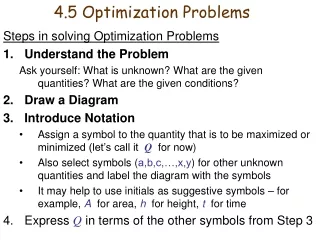
Optimization Problems
Optimization is crucial in solving complex problems in real-world scenarios such as the Traveling Salesman Problem and chess. It aims to find the optimal solution with the minimum cost. This encompasses both static optimization, where constraints remain fixed, and dynamic optimization, where constraints change over time. Techniques like Genetic Algorithms (GA), adaptive GA, and hybrid approaches enhance problem-solving capabilities. Applications range from vehicle routing to large-scale scheduling, revealing the importance of adaptive strategies in handling evolving conditions effectively.

Optimization Problems
E N D
Presentation Transcript
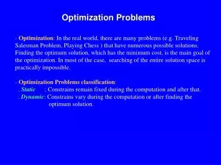
Optimization Problems • Optimization: In the real world, there are many problems (e.g. Traveling Salesman Problem, Playing Chess ) that have numerous possible solutions. • Finding the optimum solution, which has the minimum cost, is the main goal of the optimization. In most of the case, searching of the entire solution space is practically impossible. • Optimization Problems classification: • . Static: Constrains remain fixed during the computation and after that. • . Dynamic: Constrains vary during the computation or after finding the • optimum solution.
Problem Solution Using Static Optimization Dynamic Optimization Correct the solution Change in problem Fig 1: Static and dynamic optimizations
Dynamic optimization • Definition: Problems constrains and elements are changed after solving • the problem. • Goal: To find the new optimum solution in the best way (the worst way • is to solve the problem from the scratch) • Current techniques: • -Using memory: Storing the history of each peak for further exploration. • - Editing the solution: Modifying the last optimum solution. • - GA (adaptive mutation): Increasing the mutation rate after each change. • - Multi-Population GA: Keep tracking of each pick by a sub-population • (i.e. an island)
Optimization Problems Applications: • Vehicle routing • Good delivery • Large scale scheduling and transportation (i.e. Army logistics) • Characteristics of dynamic optimization environments: • Elements and conditions change by the time. • Optimum solution change by the time. • Computation time is high. • Example: • Traveling Salesman Problem (TSP) for Good delivery
Genetic Algorithms, strength and drawbacks GA : Inspiring from genetic engineering to improve a generation of the chromosomes (i.e. solutions) and result excellent genomes (i.e. solutions). Solution 1 Generation 1 Generation 2 Generation m Chromosome 1 Chromosome 2 Chromosome n Chromosome 1 Chromosome 2 Chromosome n Chromosome 1 Chromosome 2 Chromosome n Evolution Xover Mutation Replacement Selection …. Fig 2: Genetic Algorithm
Why GA for optimization ? GA is Able to cover the solution space widely Easy to hybrid with other algorithms (e.g. Local search) Flexible and suitable for dynamic environments Limitations of basic GA . Still no guarantee for optimum solution (i.e. premature convergence) . High computation time
Advanced GA Adaptive GA: Auto adjusting the GA operators according the evaluation of the chromosomes in each generation Initialization Evolution of individuals Next generation Evaluation of convergence rate Final solution GA Parameters adjustment Fig 3: Adaptive GA
Advanced GA (Cont.) Parallel GA: - Independent/Dependent multi-population GA - Synchronized/Synchronized PGA - P2P/Master-slave sup-populations Problem Sub Population n Sub Population 1 Sub Population 2 …. Best solution Fig 4: Parallel GA
Advanced GA (Cont.) Hybrid GA: Using a greedy algorithm (i.e. Local Search) to improve the quality of individuals in each generation Initialization Evolution of individuals by GA Next generation Exploitation by heuristic search Evaluation of individuals by GA Final solution Fig 5: Hybrid GA
Advanced GA (Cont.) Multi-level GA: Splitting the problem into the small sub-problems and merging the sub-solutions Original problem Clustering Sub-problem 1 Sub-problem 2 Sub-problem 3 Sub-population 1 Sub-population 2 PGA Sub-population 3 Merging Master Population Final solution Fig 6: Multi Level GA
IGA for optimization What is IGA (Island-based GA) ? IGA is a multi-population GA in which chromosomes can migrate between the islands (sup-population). Island 1 migration Island 3 Island n Island 2 Fig 7: Island Based GA
IGA for optimization • IGA (Island-based GA) characteristics: • Customized multi-population (i.e. Islands) • Synchronized and P2P migration (i.e. ring topology) • Adaptive operators: • - Local operators (mutation, crossover and hybrid rate) • - Global operators (migration rate, migration period) • Selectable hybrid (e.g. GA+LS, GA+TS, GA+SA) • Using two method crossovers dynamically (i.e. one and two point) • Auto-controlling “Occurrence” of each chromosomes to prevent the • saturation of the population.
Injection starts and stops periodically Tour Cost Pop 1 (without remote injection) Pop 2 (without remote injection) Pop 1 (with remote injection) Pop 2 (with remote injection) Generation no Fig 8: Periodically remote chromosomes injection prevents a common convergence
Initial global variables Read the benchmark Receive the best solution so far from each island Calculate the costs Islands Start Show the results Generate the islands Has the last island sent the results ? Send the global variables to each island No Run islands in parallel Yes Stop Fig 9: IGA main algorithm
Initial the population Selection Cross over and mutation Send the best individual to the controller New population Local search Migration (send/receive chromosome) Evaluation of population & parameters adjustment Fig 10: IGA algorithm for an island
Advantages of IGA • Due to multi-population characteristic of IGA, the possibility of • getting stuck with local optimums is less in IGA than a single-population GA. • For lowering the computation time, each island may reside on a machine. • Periodically migration of chromosomes between the islands lowers chance of • premature convergence. • Adaptive operators, improve the performance. • Using a multi-method algorithm (i.e. hybrid) takes most advantage of the different • search techniques. • Each island can use different operator values (population size, mutation • rate and etc). This increases the diversity of the chromosomes and • decreases similarity of the islands. • PGA are more flexible when dealing with dynamic environments. • IGA has a better performance (i.e. in terms of quality of results) than • regular PGA.
Implementation and results so far • Using TSP as Benchmark • Evaluating and tuning the GA operators in static benchmarks, including: • - Local operator: Mutation and Crossover rates • - Hybrid operators: Method and rates • - Global operators: Rate and period of immigration and no. of islands • Creating a “Dynamic benchmark generator” that can periodically change • the distances between the cities • Observation of the system reactions (best fitness) to the dynamic • changes
Implementation and results so far (Cont.) • Generalizing the optimum values of the operators from static to the • dynamic environment • Evaluating the performance of the algorithm (results) by a factor (i.e. • improvement average cost) that has a consistent values, in addition to • “Best cost”, which is random • A visualized output for evaluation of the algorithm • Evaluation of adaptive parameters
Evaluation of IGA • For evaluation of IGA two comparisons have been done: • Comparison of pure and hybrid IGA (quality and Computation time) to • verify the preferred algorithm. • Comparison of IGA with the traditional searching methods, in terms of • quality of the results and computation time, to evaluate the performance of • the IGA.
Comparison between IGA and other methods Current Heuristic Methods: Local Search (LS): A greedy algorithm that considers the best first change in the solution. Simulating Annealing (SA): An algorithm that refers to the simulation technique in conjunction with an annealing (i.e. cooling) schedule of declining temperature. Tabu search (TS): An algorithm similar to LS plus using memory to avoid repeating moves.
Fig 16: No. of Islands evaluation in terms of CPU time (IGA)
Results analysis and conclusion • Multi-population GA ,including IGA, have a better performance • compared with single-population GA. • Using a hill-climbing (i.e. Local search) method with GA (Hybrid GA), • improves the results considerably. • Migration of chromosomes lowers a premature convergence. • IGA can handle dynamic optimization problems better than plain • (single population) GA. • Optimum values for migration parameters (i.e. rate and period) • and also for number of the islands can be obtained for each benchmark.
Results analysis and conclusion (Cont.) • Variable crossover (one/two point) is better than fixed crossover. • Independent characteristic of the islands and cooperation among them can • handle changes in a dynamic benchmark better. • IGA has a better performance than traditional search methods (e.g. Local • Search, Tabu Search , Simulating Annealing) in term of efficiency (i.e. • quality of the results and considerable CPU time). • Migration in IGA helps to handle large benchmarks better.