Theorems on Redundancy Identification
230 likes | 247 Vues
This paper discusses the problem of identifying logic redundancy and presents the completion of a previous implementation, along with the fixed-value theorem and stem unobservability theorems. Results and conclusions are provided.

Theorems on Redundancy Identification
E N D
Presentation Transcript
Theorems on Redundancy Identification Vishal J. Mehta Vishwani D. Agrawal Michael L. Bushnell Rutgers University, ECE Dept. Piscataway, New Jersey, USA Mehta et al.: Redundancy theorems
Talk Outline • Introduction • Problem statement • Prior work • Primary contribution • Completion of previous implementation • Fixed-value theorem • Stem unobservability theorems • Results and conclusion Mehta et al.: Redundancy theorems
Problem Statement For identifying logic redundancy: • Implement the implication graph and transitive closure procedures with direct and partial implications. • Enhance transitive closure for contrapositive implications and fixed-valued signals. • Find new ways to Identify unobservable fanout stems. Mehta et al.: Redundancy theorems
Prior Work on Redundancy • Automatic Test Pattern Generation (ATPG) • Uses exhaustive test pattern generation to determine whether or not a target fault has a test. • Can identify all redundancies -- exponential complexity. • Boolean satisfiability methods use logic implications: Chakradhar et al., Larrabee, Henftling et al., Zhao et al., etc.. • Testability analysis (fault-independent) • Mostly approximate, linear complexity • Raitu et al., Goldstein, Seth and Agrawal, etc. • Fault-independent redundancy identification • Implication analysis identifies all or a subset of redundant faults -- polynomial complexity (empirically linear). • Agrawal et al., Gaur et al., Iyer and Abramovici, etc. Mehta et al.: Redundancy theorems
Fault-Independent Methods • Iyer and Abramovici (IEEE-TC, June 1996) use implications to find redundant faults whose tests require contradictory values on a signal. • Agrawal et al. (ATS’96) use implication graph, introduce observability variables, and use transitive closurefor redundancy identification. • Gaur et al. (DELTA’02) include anding nodes to represent higher-order implications among signals and observability variables. Mehta et al.: Redundancy theorems
Od Oc Redundancy Identification by Transitive Closure c a b c d a s-a-0 e s-a-0 b d Circuit with two redundant faults TC graph (some nodes and edges not shown) Implication Partial implication Transitive closure edge Mehta et al.: Redundancy theorems
Method Summarized • Obtain an implication graph from the circuit topology and compute transitive closure. • There are 8 different conditions on the basis of which a fault is identified to be redundant. • Examples: • If node c implies c then line c is fixed at 0 and s-a-0 fault on it is redundant. • If node Oc implies Oc then line c is unobservable and both s-a-0 and s-a-1 faults on it are redundant. • These conditions obey the contrapositive rule. Mehta et al.: Redundancy theorems
Talk Outline • Introduction • Problem statement • Prior work • Primary contribution • Completion of previous implementation • Fixed-value theorem • Stem unobservability theorems • Results and conclusion Mehta et al.: Redundancy theorems
Motivation • Incomplete implementation (Gaur et al.) • Only few anding nodes implemented • Some direct implications missing • Not all contrapositive relations determined by transitive closure • Effect of fixed-valued nodes not included in transitive closure • No observability relation across fanouts • Redundancies due to stem unobservability not identified Mehta et al.: Redundancy theorems
Completion of Previous Implementation • Only one of the possible (n+1) signal anding nodes were implemented by Gaur et al. • None of the possible n(n+1) observability anding nodes were implemented. • Some direct implications for observability variables were not implemented. Mehta et al.: Redundancy theorems
Oa1 a c d b Example Circuit a1 s-a-0 a d • Gaur et al. identified b1 s-a-1 and d s-a-0, but could not identify a1 s-a-0, because of unimplemented anding node for gate d. s-a-1 e b s-a-0 b1 c Note: only some nodes and edges are shown. Mehta et al.: Redundancy theorems
Fixed-Value Theorem • If a Boolean variable in the implication graph is fixed to a true (false) value then there exist unconditional edges from all other nodes in the graph to the node representing the true (false) state of the fixed variable. Mehta et al.: Redundancy theorems
s-a-1 s-a-1 s-a-0 s-a-1 e g e s-a-1 f f g s-a-0 s-a-1 e f g Example Circuit Note: Only some edges are shown • Initially only 2 out of 7 redundant faults were identified. • After the implementation of node fixation concept, • g-(s-a-1) was identified. • With stem unobservability theorems, rest of the 4 • redundant faults were identified. Mehta et al.: Redundancy theorems
Stem Unobservability Theorem 1 • A fanout stem is unobservable, if each signal in its dominator set assumes a constant value and: • either the fanout stem does not hold a constant value • or the fanout stem holds a constant value and, in spite of any local change in the stem signal, the dominator set values do not change. Notes: • A local change of a signal only affects the portion of the circuit between that signal and POs. • Dominator set is the set of signals through which a signal in the circuit should pass in order to reach the primary output. Mehta et al.: Redundancy theorems
a c 1 d b unobs. stem fixed dom. Example Circuit • For the fanout stem b, the dominator signal d is fixed to 1. • As b is not fixed, Theorem 1 identifies b as unobservable stem. Mehta et al.: Redundancy theorems
Theorem 2 • A fanout stem is unobservable, if each signal in its dominator set is unobservable and: • either the stem does not hold a constant value • or the stem holds a constant value and, in spite of any local change in the stem signal, the unobservable status of the dominator set remains unchanged. Note: A lemma by Iyer and Abramovici is a special case of Theorem 2. Mehta et al.: Redundancy theorems
c 0(fixed) a d b1 unobs. unobs. e b Example Circuit • Fixed value 0 on line c makes the fanout branches b1 and b2 of stem b unobservable. • As b is not fixed, Theorem 2 identifies b as an unobservable stem. Note: Stem a is unobservable by Theorem 1, which does not classify stem c as unobservable. b2 unobs. Mehta et al.: Redundancy theorems
Talk Outline • Introduction • Problem statement • Prior work • Primary contribution • Completion of previous implementation • Fixed-value theorem • Stem unobservability theorems • Results and conclusion Mehta et al.: Redundancy theorems
Benchmark Results Identified redundant faults and computation time Circuit C5315 c2670 s9234 s s13207 Total Flts. 5350 2747 6927 9 9815 • ATPG • Flts. CPU s • 59 32.3 • 115 95.2 • 452 803.7 • TCSTEM • Flts. CPU s • 58 3.9 • 82 4.0 • 233 106.0 • TCAND • Flts. CPU s • 32 3.4 • 25 1.5 • 135 11.2 • FIRE • Flts. CPU s • 20 2.8 • 29 1.5 • 165 20.6 60 13.6 151 806.5 77 158.8 55 23.2 ATPG: TRAN, Chakradhar et al., IEEE-TCAD’93, Sparc 5 TCSTEM: This work, Sparc 5 TCAND: Gaur et al., DELTA’02, Sparc 5 FIRE: Iyer and Abramovici, IEEE-TVLSI’96, Sparc 2 Mehta et al.: Redundancy theorems
s-a-1 unobs. stem a e s-a-1 a d f s-a-1 h c f b b e d s-a-0 g c s-a-1 s-a-1 Limitations of Method • Example 1: None of the stem unobservability theorems can identify stem a as unobservable because the dominator set is neither fixed nor unobservable. • Example 2: e s-a-1 is redundant because f=g=1 require b=0, which implies e=1. Because f=1 and g=1 are separately treated in the transitive closure and each has multiple satisfying choices, the essential requirement b=0 is not found. The method fails to find this redundancy. Example 2 Example 1 Mehta et al.: Redundancy theorems
Conclusion • Partial implications, fixed-value theorem and stem unobservability theorems improve the process of redundant fault identification better than any other known fault-independent technique. • Checking for the contrapositive rule to update transitive closure may have benefits. • A demonstrated limitation of stem unobservability theorems can be improved upon. • Possible ways to find essential signal assignments caused by combinations of multiple signals may provide further improvements. Mehta et al.: Redundancy theorems
Future Work • Various applications of the TC technique can be explored: • Identifying equivalent faults • Checking equivalence of combinational circuits. • 2 and 3 valued logic simulators. Mehta et al.: Redundancy theorems
THANK YOU Mehta et al.: Redundancy theorems