Redundancy

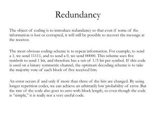
1. Redundancy • The object of coding is to introduce redundancy so that even if some of the information is lost or corrupted, it will still be possible to recover the message at the receiver. • The most obvious coding scheme is to repeat information. For example, to send a 1, we send 11111, and to send a 0, we send 00000. This scheme uses five symbols to send 1 bit, and therefore has a rate of 1/5 bit per symbol. If this code is used on a binary symmetric channel, the optimum decoding scheme is to take the majority vote of each block of five received bits. • An error occurs if and only if more than three of the bits are changed. By using longer repetition codes, we can achieve an arbitrarily low probability of error. But the rate of the code also goes to zero with block length, so even though the code is “simple,” it is really not a very useful code.

2. Error Detecting Codes • We can combine the bits in some intelligent fashion so that each extra bit checks whether there is an error in some subset of the information bits. • A simple example of this is a parity check code. Starting with a block of n − 1 information bits, we choose the nth bit so that the parity of the entire block is 0 (the number of 1’s in the block is even). • Then if there is an odd number of errors during the transmission, the receiver will notice that the parity has changed and detect the error. • This is the simplest example of an error-detecting code. The code does not detect an even number of errors and does not give any information about how to correct the errors that occur.

3. Hamming Code • We can extend the idea of parity checks to allow for more than one parity check bit and to allow the parity checks to depend on various subsets of the information bits. The Hamming code is an example of a parity check code. • We consider a binary code of block length 7. Consider the set of all nonzero binary vectors of length 3. Arrange them in columns to form a matrix: • Consider the set of vectors of length 7 in the null space of H (the vectors which when multiplied by H give 000). The null space of H has dimension 4.

4. Minimum Weight • 24 codewords: • Since the set of codewords is the null space of a matrix, it is linear in the sense that the sum of any two codewords is also a codeword. The set of codewords therefore forms a linear subspace of dimension 4 in the vector space of dimension 7. • Looking at the codewords, we notice that other than the all-0 codeword, the minimum number of 1’s in any codeword is 3. This is called the minimum weight of the code.

5. Minimum Distance • We can see that the minimum weight of a code has to be at least 3 since all the columns of H are different, so no two columns can add to 000. • The fact that the minimum distance is exactly 3 can be seen from the fact that the sum of any two columns must be one of the columns of the matrix. • Since the code is linear, the difference between any two codewords is also a codeword, and hence any two codewords differ in at least three places. The minimum number of places in which two codewords differ is called the minimum distance of the code.

6. Minimum Distance • The minimum distance of the code is a measure of how far apart the codewords are and will determine how distinguishable the codewords will be at the output of the channel. • The minimum distance is equal to the minimum weight for a linear code. We aim to develop codes that have a large minimum distance. • For the code described above, the minimum distance is 3. Hence if a codeword c is corrupted in only one place, it will differ from any other codeword in at least two places and therefore be closer to c than to any other codeword. • But can we discover which is the closest codeword without searching over all the codewords?

7. Parity Check Matrix • The answer is yes. We can use the structure of the matrix H for decoding. The matrix H, called the parity check matrix, has the property that for every codeword c, Hc = 0. • Let eibe a vector with a 1 in the ith position and 0’s elsewhere. If the codeword is corrupted at position i, the received vector r = c + ei. If we multiply this vector by the matrix H, we obtain: • which is the vector corresponding to the ith column of H. Hence looking at Hr, we can find which position of the vector was corrupted. Reversing this bit will give us a codeword.

8. Error Correction • This yields a simple procedure for correcting one error in the received sequence. We have constructed a codebook with 16 codewords of block length 7, which can correct up to one error. This code is called a Hamming code. • We have to define now an encoding procedure; we could use any mapping from a set of 16 messages into the codewords. But if we examine the first 4 bits of the codewords in the table, we observe that they cycle through all 24 combinations of 4 bits. • Thus, we could use these 4 bits to be the 4 bits of the message we want to send; the other 3 bits are then determined by the code.

9. Systematic Code • In general, it is possible to modify a linear code so that the mapping is explicit, so that the first k bits in each codeword represent the message, and the last n − k bits are parity check bits. Such a code is called a systematic code. • The code is often identified by its block length n, the number of information bits k and the minimum distance d. For example, the above code is called a (7,4,3) Hamming code (i.e., n = 7, k = 4, and d = 3). • An easy way to see how Hamming codes work is by means of a Venn diagram. Consider the following Venn diagram with three circles and with four intersection regions as shown in Figure (Venn-Hamming 1).

10. Venn Representation • To send the information sequence 1101, we place the 4 information bits in the four intersection regions as shown in the figure. We then place a parity bit in each of the three remaining regions so that the parity of each circle is even (i.e., there are an even number of 1’s in each circle). Thus, the parity bits are as shown in Figure (Venn-Hamming 2) Venn-Hamming 1 Venn-Hamming 2

11. Venn Representation • Now assume that one of the bits is changed; for example one of the information bits is changed from 1 to 0 as shown in Figure Humming-Venn 3. • Then the parity constraints are violated for two of the circles, and it is not hard to see that given these violations, the only single bit error that could have caused it is at the intersection of the two circles (i.e., the bit that was changed). Similarly working through the other error cases, it is not hard to see that this code can detect and correct any single bit error in the received codeword.

12. Generalization • We can easily generalize this procedure to construct larger matrices H. In general, if we use l rows in H, the code that we obtain will have block length n = 2l − 1, k = 2l − l − 1 and minimum distance 3. All these codes are called Hamming codes and can correct one error. • Hamming codes are the simplest examples of linear parity check codes. But with large block lengths it is likely that there will be more than one error in the block. • Several codes have been studied: t-error correcting codes (BCH codes), Reed-Solomon codes that allow the decoder to correct bursts of up to 4000 errors.

13. Block Codes and Convolutional Codes • All the codes described above are block codes, since they map a block of information bits onto a channel codeword and there is no dependence on past information bits. • It is also possible to design codes where each output block depends not only on the current input block, but also on some of the past inputs as well. • A highly structured form of such a code is called a convolutional code. • We will discuss Reed-Solomon and convolutional codes later.

14. A Bit of History • For many years, none of the known coding algorithms came close to achieving the promise of Shannon’s channel capacity theorem. • For a binary symmetric channel with crossover probability p, we would need a code that could correct up to np errors in a block of length n and have n(1 − H(p)) information bits (which corresponds to the informative capacity of the channel). • For example, the repetition code suggested earlier corrects up to n/2 errors in a block of length n, but its rate goes to 0 with n. • Until 1972, all known codes that could correct nα errors for block length n had asymptotic rate 0.

15. A Bit of History • In 1972, Justesen described a class of codes with positive asymptotic rate and positive asymptotic minimum distance as a fraction of the block length. • In 1993, a paper by Berrou et al. introduced the notion that the combination of two interleaved convolution codes with a parallel cooperative decoder achieved much better performance than any of the earlier codes. • Each decoder feeds its “opinion” of the value of each bit to the other decoder and uses the opinion of the other decoder to help it decide the value of the bit. This iterative process is repeated until both decoders agree on the value of the bit. • The surprising fact is that this iterative procedure allows for efficient decoding at rates close to capacity for a variety of channels.

16. LDPC and Turbo Codes • There has also been a renewed interest in the theory of low-density parity check (LDPC) codes that were introduced by Robert Gallager in his thesis. • In 1997, MacKay and Neal [368] showed that an iterative message-passing algorithm similar to the algorithm used for decoding turbo codes could achieve rates close to capacity with high probability for LDPC codes. • Both Turbo codes and LDPC codes remain active areas of research and have been applied to wireless and satellite communication channels. • We will discuss LDPC and Turbo codes later in this course.

17. Feedback Capacity • A channel with feedback is illustrated in Figure. We assume that all the received symbols are sent back immediately and noiselessly to the transmitter, which can then use them to decide which symbol to send next. • Can we do better with feedback? The surprising answer is no.

18. Feedback Code • We define a (2nR, n) feedback code as a sequence of mappings xi(W, Y i−1), where each xiis a function only of the message W ∈ 2nRand the previous received values, Y1, Y2, . . . , Y i−1, and a sequence of decoding functions g : n→ {1, 2, . . . , 2nR}. Thus, • Pe(n)= Pr{g(Yn) ≠ W} • when W is uniformly distributed over {1, 2, . . . , 2nR}. • DefinitionThe capacity with feedback, CFB, of a discrete memoryless channel is the supremum of all rates achievable by feedback codes.

19. Feedback Capacity and C • Theorem (Feedback capacity) • As we have seen in the example of the binary erasure channel, feedback can help enormously in simplifying encoding and decoding. However, it cannot increase the capacity of the channel.

20. Source-Channel Separation • It is now time to combine the two main results that we have proved so far: data compression (R >H) and data transmission (R < C). • Recall that the first is provided by the relationship between the entropy rate H() and the expected number of bit per symbol Ln* required to describe a stochastic process. • Is the condition H <C necessary and sufficient for sending a source over a channel? • For example, consider sending digitized speech or music over a discrete memoryless channel. We could design a code to map the sequence of speech samples directly into the input of the channel, or we could compress the speech into its most efficient representation, then use the appropriate channel code to send it over the channel.

21. Source-Channel Separation • It is not immediately clear that we are not losing something by using the two-stage method, since data compression does not depend on the channel and the channel coding does not depend on the source distribution. • We will prove in this section that the two-stage method is as good as any other method of transmitting information over a noisy channel. • It implies that we can consider the design of a communication system as a combination of two parts, source coding and channel coding. • We can design source codes for the most efficient representation of the data. We can, separately and independently, design channel codes appropriate for the channel. The combination will be as efficient as anything we could design by considering both problems together.

22. It is so Obvious? • The result that a two-stage process is as good as any one-stage process seems obvious, however, there are interesting examples to see that it is not. • A simple example is that of sending English text over an erasure channel. We can look for the most efficient binary representation of the text and send it over the channel. But the errors will be very difficult to decode. If, however, we send the English text directly over the channel, we can lose up to about half the letters and yet be able to make sense out of the message. • Similarly, the human ear has some unusual properties that enable it to distinguish speech under very high noise levels if the noise is white. In such cases, it may be appropriate to send the uncompressed speech over the noisy channel rather than the compressed version. • Apparently, the redundancy in the source is suited to the channel.

23. Formalization • Let us define the setup under consideration. We have a source V that generates symbols from an alphabet V. We will not make any assumptions about the kind of stochastic process produced by V other than that it is from a finite alphabet and satisfies the AEP (an example is the sequence of states of a stationary irreducible Markov chain). • We want to send the sequence of symbols V n= V1, V2, . . . , Vnover the channel so that the receiver can reconstruct the sequence. To do this, we map the sequence onto a codeword Xn(V n) and send the codeword over the channel. • The receiver looks at his received sequence Ynand makes an estimate ˆV nof the sequence V n that was sent. The receiver makes an error if V n≠ ˆV n.

24. Formalization • We define the probability of error as: • Where I is the indicator function and g(yn) is the decoding function.

25. Source-Channel Coding Theorem • Theorem (Source–channel coding theorem) If V1, V2, . . . Vn is a finite alphabet stochastic process that satisfies the AEP and H() < C, there exists a source–channel code with probability of error Pr( ˆV n ≠ V n)→ 0. • Conversely, for any stationary stochastic process, if H() > C, the probability of error is bounded away from zero, and it is not possible to send the process over the channel with arbitrarily low probability of error.

26. Comments • Hence, we can transmit a stationary ergodic source over a channel if and only if its entropy rate is less than the capacity of the channel. • The joint source–channel separation theorem enables us to consider the problem of source coding separately from the problem of channel coding. The source coder tries to find the most efficient representation of the source, and the channel coder encodes the message to combat the noise and errors introduced by the channel. • The separation theorem says that the separate encoders can achieve the same rates as the joint encoder.

27. The data compression theorem is a consequence of the AEP, which shows that there exists a “small” subset (of size 2nH) of all possible source sequences that contain most of the probability and that we can therefore represent the source with a small probability of error using H bits per symbol. • The data transmission theorem is based on the joint AEP; it uses the fact that for long block lengths, the output sequence of the channel is very likely to be jointly typical with the input codeword, while any other codeword is jointly typical with probability ≈ 2−nI. Hence, we can use about 2nI codewords and still have negligible probability of error. • The source–channel separation theorem shows that we can design the source code and the channel code separately and combine the results to achieve optimal performance.