Download
1 / 35
360 likes | 513 Vues
The Carbon Cycle. Oral review presentation, 2004 Chengyuan Xu. Outline. Anthropogenic time scale (<10 3 yr) Glacial – Interglacial variation (10 3 -10 5 yr) Geological scale (>10 8 yr). Faint Young Sun Paradox.

E N D
The Carbon Cycle Oral review presentation, 2004 Chengyuan Xu
Outline • Anthropogenic time scale (<103yr) • Glacial – Interglacial variation (103-105yr) • Geological scale (>108yr)
Faint Young Sun Paradox • Sun’s energy was 30% lower 4.6 Bys ago (H fused to He, so more energy generation is required to compensate the decrement of thermal pressure) • Liquid water existed on earth for 3.8 Bys(sediment), indicating constant earth temperature • Some temperature regulator
Global Carbon Cycle at Geological Scale Organic C
A model of long-term carbon cycle CO2+CasiO3 CaCO3+SiO2 (1)* CO2+H2O CH2O+O2 (2)
BLAG Scenario Atm CO2 increase Global Climate Change: Atm CO2 decrease Warmer New Balance Wetter CaSiO3 Soil CO2 increase
To Test the Scenario • Outgassing CO2 should equal CaCO3 subducted • Calcium input from terrestrial silicates should balance air CO2 deposited • The sea floor spread was much faster 1 Mys ago (Pittman and Hays), so there should be more CO2 outgassing. More CaCO3 sediments and weathering was expected to maintain the balance of carbon. • Warmer 1 Mys ago • Higher atmosphere CO2 concentration 1 Mys ago
Ca-CO2 Balance • Carbon outgassing and subducted is far from effectively measurable • The error of Calcium flux to ocean is too large for reliable evaluation of the scenario • Only 20±5% of Ca2+ is from silicates, others are from limestone, causing and error bar of 100% in measurement • Can not partition
Globally Bulk earth carbon and sediment carbon: δ13C = -5‰ Organic material: δ13C = -25‰ Limestone carbon: δ13C = -25‰ -5‰(1.0) = (1-X) (-25‰) + X(0‰) X = 0.8 In river Rivers draining limestone terrane δ13C (HCO3-)= -13‰ Rivers draining silicate terrane: δ13C (HCO3-)= -26‰ Organic derived CO2: δ13C = -26‰ Exchange with Atm CO2: δ13C = -8‰ Use carbon isotope to estimate of gassed CO2 from limestone vs from organic materials
Estimating Weathering rate • Use 87Sr/87Sr in foraminifera, which reflects ocean 87Sr/87Sr • Terrestrial derived Sr is more 87Sr enriched than hydrothermal ridge derived Sr • Unfortunately, the elevated 87Sr/87Sr since 40 Mys ago was caused by the rise of Himalaya, which brings 87Sr enriched Sr to continent
Polar Ocean Temperature since Cretaceous • Oxygen isotope ratios in benthic foraminfera reflect 18O/17O ratio in ocean • Fractionation during evaporation • The colder, the fewer water remain in ocean, so ocean is 18O in enriched
Marine Phytoplankton Carbon fractionation occurs during photosynthesis and the extent is determined by the CO2 dissolved in the surface water Temperature and some other influential factors can be regulated 1000 ppm CO2 during 100 myrs ago Soil caliche (CaCO3) Partition the source of caliche into organic derived CO2 and air CO2 by δ13C Get atm [CO2]: soil [CO2], assuming soil CO2 does not change much 100 myrs ago, [CO2] is about an order of magnitude grater than today Paleo Atm CO2 indicator: δ13C
Venus So much CO2 accumulate in the atmosphere that water evaporated before feedback works No sediment can form and the regulation ends 430°C at surface Snowball So few CO2 stay in atmosphere that temperature drop below to –80°C All CO2 outgassed become dry ice Fortunately, the earth escaped the fate at least twice Scenarios of Venus and Snowball
Long Term CO2 Record Spread of vascular plants 550myrs “Snow Ball Earth” Event 440myrs First land plant 400myrs First tree like plant 360myrs First Soil Large glacial event
Glacial-Interglacial CO2 variation • Vostok ice core in Antarctic showed 80ppm CO2 rise (200 to 280) when glacial era ends (till 400,000 years ago) • Ice core in Dansgarard-Oeschgar is Greenland was contaminated by acid released CO2 from CaCO3
CO2 inventory during glacial era • Interglacial Glacial • Atmosphere CO2 decrease 80 ppm • Terrestrial biome carbon sink decrease 500 Gt (1015g), equaling inject 56 ppm CO2 to atmosphere, among which 40 ppm is absorbed by ocean* • 2 °C cooling in North Atlantic decrease atmosphere CO2 by 20 ppm • Salinity increase 3%, raising CO2 for 10 ppm • In all, we need to explain about 80 ppm CO2 decline
Biological Pump • Nutrient limits productivity in ocean • Fe:P:N:C =1:1000:16000:125000
Iron Fertilization • Higher dust input to ocean during glacial • High Fe facilitated cynaobacteria in the tropic, which fix N • Several thousand years lag between dust decline and temperature increase • Ligand combined iron
Explanation of constant carbon isotope in ocean inorganic carbon • Photosynthesis fractionation elevate 13C/12C ratio in surface ocean inorganic carbon • High 13C/12C ratio indicates higher nutrient utilization (productivity) Terrestrial carbon input Temperature and pH dependent
Ocean Inorganic Carbon Pool and Lysocline • In ocean, [CO2] ≈ 1/[CO32-] • So dissolution of CaCO3 can decreased pCO2 • Lysocline marks the depth below which CaCO3 will dissolve • Lysocline is supposed to decline for 3000 meters if CO2 decrease 80 ppm, but we observed on 800m • Respiration of bacteria at ocean bottom can also dissolve CaCO3 and may decouple the relationship • Supported by paleo pH proxy (B(OH)3/B(OH)4-), pH increased 0.3 and [CO32-] doubled • Biological pump can increase organic C deposition and breed bacteria
Other Scenarios • Coral Reef generation decreased during glacial era due to the decline of sea level and more coral exposed to air subjecting to erosion • Lower marine organism calcite production, perhaps due to the competition advance of diatom • Due to more freeze-thaw activity, more alkalinity input into ocean which increase [CO32-]
Anthropogenic led CO2 increase • Seasonal oscillation – vegetation phenology • Increased mplitude – CO2 and N fertilization • Flattening – photosynthesis and ocean absorption
Source Respiration Ocean release Fossil fuel Deforestation Methane Missing Carbon: 2.8 Gt CO2 fertilization N fertilization Forest regeneration Global Carbon Balance • Sink • Atmosphere • Ocean • Terrestrial vegetation • Soil • Rock
Fossil Fuel • Coal: buried in anoxic environments, 300-400years usage • Oil/Natural gas:buried in sedimentary layer, enriched in porous medium, 85/35 years usage • High temperature and pressure for millions of years • 13C and 14C depleted
Basic Reactions • Photosynthesis 6CO2+12H2*OC6H12O6+6*O2+6H2O • Respiration C6H12O6+6O26CO2+6H2O • Ocean absorption of CO2 CO2+CO32-+H2O2HCO3- CO2+H4BO4-HCO3-+H3BO3 • Weathering in soil CO2+H2OH2CO3H++HCO3-
The Role of the Ocean • Turnover rate about 1000 years, can uptake 5/6 of the fossil CO2 • Currently, uptake about 50% (2-3Gt) • The Revelle rate: The percentage increase of atm CO2 required to raise the total CO2 inventory by one percent (on the order of 9-14%)
Modeling Ocean Uptake of CO2 • CO2 exchange rate (natural and bomb 14C, Radon) • Thickness of mixed layer (wave) • Eddy diffusivity (bomb 3H and 14C penetration in ocean) • The extent of vertical mixing varies as the square root of time Atmosphere CO2 exchange rate (0.064mol m-2 yr-1μatm-1 ) Ocean Mixed Layer 75m Ocean Interior Eddy Diffusivity 2.4cm2s-1
Model Results • Uptake 2 Gt Carbon per year • Average penetration of 380 m in ocean • Bomb 14C is the best tracer for setting the gas exchange rate and the coefficient of eddy diffusivity
Other Scenarios • Use gas exchange rate and air-ocean pCO2 gradient to estimate CO2 uptake – too large error bar (4± 4 ppm difference, 8ppm equals 2Gt uptake)
Interhemisphere CO2 gradient • Increased gradient since 1950 • Higher CO2 in South hemisphere before 1950 • Excess CO2 carried by NADW to Antarctic (0.6Gt) • Respiration and nutrients (P)
Terrestrial Carbon Sink • Photosynthesis reaction to CO2 • Acclimation • In general, 3-3.5% growth increment per 10% [CO2] increment • Nitrogen fertilization
Leaf 2yrs Model 150Gt 0.2Gt/yr Wood 60yrs 500Gt 0.3Gt/yr • 1.1 Gt in all for CO2 fertilization mainly in North America and Euroasia • 0.5 Gt for Nitrogen fertilization Active Soil 15 yrs 75% 500Gt 0.5Gt/yr Inert Soil 3500 yrs Additionally, 0.04Gt N fertilization/yr and C/N=12
Artificial CO2 Sequestion (by Klaus Lackner) • Tie up CO2 into stable chemical forms and can safely deposit them. • Reactions CO2+CaOCaCO3 CaCO3+MgOMgCO3+CaO • Air masses flow and come into contact with the sorbent and subsequently remove CO2 gas from the atmosphere • 60km3 MgCO3, a mountain, crazy idea