Download
1 / 14
180 likes | 901 Vues
The Biogeochemical Sulfur Cycle. Contents. Introduction The global sulfur cycle Sulfur isotopes Example: the use of sulfur isotopes to predict the early history of atmospheric oxygen. Introduction. Sulfur 14th most abundant element Reduced FeS 2 (-2 or –1) Oxidized SO 4 2- (+6)

E N D
Contents • Introduction • The global sulfur cycle • Sulfur isotopes • Example: the use of sulfur isotopes to predict the early history of atmospheric oxygen
Introduction • Sulfur 14th most abundant element • Reduced FeS2 (-2 or –1) • Oxidized SO42- (+6) • Intermediate valences can occur (transitory)
Four stable isotopes: 32S, 33S, 34S and 36S Abundance 95 %, 0.76 %, 4,22 %, 0,014% Standard: Canyon Diablo Troilite (CDT, a meteorite) 34S (‰) = (34S/32S)sample -1/ (34S/32S)CDT x 1000 Sulfur Isotopes
Fractionation mechanisms • Exchange reactions between sulfates and sulfides. • Kinetic isotopic effects in the bacterial reduction of sulfate. • Precipitation of sulfates in seawater.
Fractionation • Organic matter oxidation by sulfate reducing bacteria (f.e. Desulfovibrio desulfuricans) CH2O + SO4 H2S + 2 HCO3- • Formation of pyrite FeS2
Example: The use of sulfur isotopes to predict the early history of atmospheric oxygen • Two scenarios: • Atm O2 reach present day levels by the earliest Archean (3.8 Ga ago). • Atm O2 began to accumulate around 2.2 /2.3 Ga in the early Proterozoic.
The sulfur isotope record • Sedimentary sulfides between 3.4 & 2.8 Ga small isotopic differences 34Ssed sulfides=5‰ against 34Ssolubl sulphate= 2-3 ‰ • Formation such sediments under high rates of sulphate reduction in a warm sulphate rich environment. • Model needs extension
Conclusion • Rapid rates of sulphate reduction with abundant SO4 and at higher temperatures up to 85°C, should produce sedimentary sulfides depleted in 34S by about 13 to 28‰ compared with seawater sulphate. • At 2.2 Ga : 34S depleted sulfides of biological origin become a continuous feature of the geological record.