Phylogenetic tree construction
Phylogenetic tree construction. Mai Nakadachi. http://libguides.scu.edu/evolution. Outline. Phylogenetic tree types Distance Matrix method UPGMA Neighbor joining Character State method Maximum likelihood. Phylogenetic tree?.

Phylogenetic tree construction
E N D
Presentation Transcript
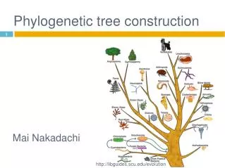
Phylogenetic tree construction Mai Nakadachi http://libguides.scu.edu/evolution
Outline • Phylogenetic tree types • Distance Matrix method • UPGMA • Neighbor joining • Character State method • Maximum likelihood
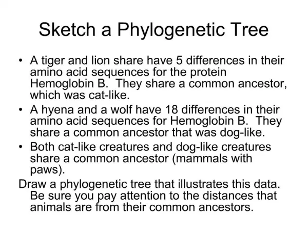
Phylogenetic tree? • A tree represents graphical relation between organisms, species, or genomic sequence • In Bioinformatics, it’s based on genomic sequence
What do they represent? • Root: origin of evolution • Leaves: current organisms, species, or genomic sequence • Branches: relationship between organisms, species, or genomic sequence • Branch length: evolutionary time (in cladogram, it doesn't represent time)
Rooted / Unrooted trees • Rooted tree: directed to a unique node • (2 * number of leaves) - 1 nodes, • (2 * number of leaves) - 2 branches • Unrooted tree: shows the relatedness of the leaves without assuming ancestry at all • (2 * number of leaves) - 2 nodes • (2 * number of leaves) - 3 branches https://www.nescent.org/wg_EvoViz/Tree
More tree types used in bioinformatics (from cohen article) • Unrooted tree • Rooted tree • Cladograms: Branch length have no meaning • Phylograms: Branch length represent evolutionary change • Ultrametric: Branch length represent time, and the length from the root to the leaves are the same https://www.nescent.org/wg_EvoViz/Tree
How to construct a phylogenetic tree? • Step1: Make a multiple alignment from base alignment or amino acid sequence (by using MUSCLE, BLAST, or other method)
How to construct a phylogenetic tree? • Step 2: Check the multiple alignment if it reflects the evolutionary process. http://genome.cshlp.org/content/17/2/127.full
How to construct a phylogenetic tree? cont • Step3: Choose what method we are going to use and calculate the distance or use the result depending on the method • Step 4: Verify the result statistically.
Distance Matrix methods • Calculate all the distance between leaves (taxa) • Based on the distance, construct a tree • Good for continuous characters • Not very accurate • Fastest method • UPGMA • Neighbor-joining
UPGMA • Abbreviation of “Unweighted Pair Group Method with Arithmetic Mean” • Originally developed for numeric taxonomy in 1958 by Sokal and Michener • Simplest algorithm for tree construction, so it's fast!
How to construct a tree with UPGMA? • Prepare a distance matrix • Repeat step 1 and step 2 until there are only two clusters • Step 1: Cluster a pair of leaves (taxa) by shortest distance • Step 2: Recalculate a new average distance with the new cluster and other taxa, and make a new distance matrix
Example of UPGMA • New average distance between AB and C is: • C to AB = (60 + 50) / 2 = 55 • Distance between D to AB is: • D to AB = (100 + 90) / 2 = 95 • Distance between E to AB is: • E to AB = (90 + 80) / 2 = 85
Example of UPGMA cont 1 • New average distance between AB and DE is: • AB to DE = (95 + 85) / 2 = 90
Example of UPGMA cont 2 • New Average distance between CDE and AB is: • CDE to AB = (90 + 55) / 2 = 72.5
Example of UPGMA cont 3 • There are only two clusters. so this completes the calculation!
Downside of UPGMA • Assume molecular clock (assuming the evolutionary rate is approximately constant) • Clustering works only if the data is ultrametric • Doesn’t work the following case:
Neighbor-joining method • Developed in 1987 by Saitou and Nei • Works in a similar fashion to UPGMA • Still fast – works great for large dataset • Doesn’t require the data to be ultrametric • Great for largely varying evolutionary rates
How to construct a tree with Neighbor-joining method? • Step 1: • Calculate sum all distance from x and divide by (leaves – 2) • Sx = (sum all Dx) / (leaves - 2) • Step 2: • Calculate pair with smallest M • Mij = Distance ij – Si – Sj • Step 3: • Create a node U that joins pair with lowest Mij • S1U = (Dij / 2) + (Si – Sj) / 2
How to construct a tree with Neighbor-joining method? • Step 4: • Join I and j according to S and make all other taxa in form of a star • Step 5: • Recalculate new distance matrix of all other taxa to U with: • DxU = Dix + Djx - Dij
Example of Neighbor-joining • Step 1: S calculation : Sx = (sum all Dx) / (leaves - 2) • S(A) = (5 + 4 + 7 + 6 + 8) / 4 = 7.5 • S(B) = (5 + 7 + 10 + 9 + 11) / 4 = 10.5 • S(C) = (4 + 7 + 7 + 6 + 8) / 4 = 8 • S(D) = (7+ 10 + 7 + 5 + 9) / 4 = 9.5 • S(E) = (6 + 9 + 6 + 5 + 8) / 4 = 8.5 • S(F) = (8 + 11 + 8 + 9 + 8) / 4 = 11
Example of Neighbor-joining cont 1 • Step 2: Calculate pair with smallest M • Mij = Distance ij – Si – Sj • Smallest are • M(AB) = d(AB) – S(A) –S(B) = 5 – 7.5 – 10.5= -13 • M(DE) = 5 – 9.5 – 8.5 = -13
Example of Neighbor-joining cont 2 • Step 3: Create a node U • S1U = (Dij / 2) + (Si – Sj) / 2 • U1 joins A and B: • S(AU1) = d(AB) / 2 + (S(A) – S(B)) / 2 = 5 / 2 + (7.5 - 10.5) / 2 = 1 • S(BU1) = d(AB) / 2 + (S(B) – S(A)) / 2 = 5 / 2 + (10.5 – 7.5) / 2 = 4
Example of Neighbor-joining cont 3 • Step 4: Join A and B according to S, and make all other taxa in form of a star. Branches in black are unknown length and Branches in red are known length
Example of Neighbor-joining cont 4 • Step5: Calculate new distance matrix Dxu = (Dix + Djx – Dij) / 2 • d(CU) = (d(AC) + d(BC) - d(AB)) / 2 • = (4 + 7 - 5) / 2 =3 • d(DU) = d(AD) + d(BD) - d(AB) / 2 = 6 Same as EU and FU • Then we get the new distance matrix
Example of Neighbor-joining cont 5 • Repeat 1 to 5 until all branches are done • In this example, we will get this at the end
Downside of Neighbor-joining • Generates only one possible tree • Generates only unrooted tree
Character state methods • Need discrete characters • Maximum likelihood • Maximum parsimony (will be covered by Kyle)
Maximum likelihood • Originally developed for statistics by Ronald Fisher between 1912 and 1922 • Therefore, explicit statistical model • Uses all the data • Tends to outperform parsimony or distance matrix methods
How to construct a treewith Maximum likelihood? • Step 1: • Make all possible trees depending on the number of leaves • Step 2: Calculate likelihood of occurring with the given data • L(Tree) = probability of each tree. • optimizing branch length • generating tree topology • Step 3: Pick the tree that have the highest likelihood.
Sounds really great? • Maximum likelihood is very expensive and extremely slow to compute
Topics • Phylogenetic tree types • Distance Matrix method • UPGMA • Neighbor joining • Character State method • Maximum likelihood