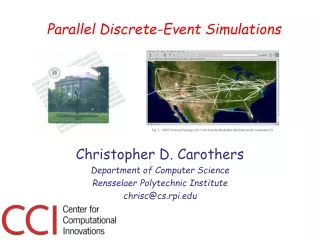
Parallel Discrete Event Simulation

1. Parallel Discrete Event Simulation Richard Fujimoto Communications of the ACM, Oct. 1990

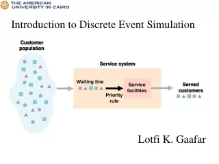
2. Introduction • Execution of a single discrete event simulation program on a parallel computer to facilitate quick execution of large simulation programs • Problems usually have substantial amount of “parallelism”. • System being simulated has states that change only at discrete instants of time, upon the occurrence of an “event”, for e.g. arrival of a message at some node in the network. • Concerns itself primarily with simulation of asynchronous systems where events are not synchronized by a global clock, i.e they are truly distributed in nature.

3. Approaches • Use dedicated functional units to implement specific sequential functions, a la vector processing • Use hierarchical decomposition of the simulation model to allow an event consisting of several sub-events to be processed concurrently. • To execute independent, sequential simulation programs on different processors, which leads to replication, which is useful if the simulation is largely stochastic. Useful only when done to reduce variance, or a specific simulation problem with different input parameters. Needs an each processor to have sufficient memory to hold an entire simulation run, potentially useless where one sequential run depends on the output of another.

4. PDES • Inherently difficult because of the typical way in which simulation is done utilizing state variables, event list and a global clock variable. • In a sequential model, the simulator runs in a loop removing the smallest time-stamped event from the event list and processes it. Processing an event means effecting a change in the system state, and scheduling zero or more new events in the simulated future in order to maintain causality relationships. • The challenging aspect of PDES is to maintain this causality relationship while exploiting inherent parallelism to schedule the jobs faster. “Maintaining” causality relationship means maintaining some sequencing order between events executing in two separate processes.

5. Strategies • Model the system as a collection of logical processes with no direct access to shared state variables. • All interactions between processes are modeled as time stamped event messages between LPs. • Causality errors can be avoided if each LP obeys its local causality constraints and interacts exclusively by exchanging time stamped messages • “Cause and effect” relationship between events must be maintained.

6. Mechanisms for PDES • Conservative Approach Avoid the possibility of any type of causality error ever occurring by determining when it is safe to process an event. Uses pessimistic estimates for decision making • Optimistic Approach Use a detection and recovery approach. Allow for causality errors, then invoke “rollback” to recover.

7. Conservative Approach • If a process P contains an unprocessed event E1 with time stamp T1 such that T1 is the smallest timestamp it has, then it must ensure that it is impossible for it to receive another event with a lower time stamp before executing E1 . • Algorithm • Statically specify links that indicate which process communicates with one another • Each process ensures that the sequence of time stamps sent over the links are increasing • Each link has a clock associated with it that is equal to the timestamp of the message at the head of the queue or the timestamp of the last received message if the queue is empty.

8. Deadlocks in Conservative Approach • Occurs when a system of empty queues exists. • Need to send messages, called “null” messages periodically, which are an assurance from each LP that the next message sent on that LP will have a timestamp greater than the null message timestamp. • A variation would be to request for null messages when all input queues to a process becomes empty. • Eliminate null messages by allowing deadlocks to occur and then breaking them by allowing the smallest time stamped event in the global state to proceed.

9. Improvements • Maintaining a simulated time window, which basically determines the number of events to be looked at for possible parallelism. • Lookahead: Ability to predict with certainty the outcome of a future event. • Conditional knowledge: Predicates are associated with events, which when satisfied imply that the event occurred. Goal is to make these events definite.

10. Performance/Shortcomings • Degree of look-ahead greatly determines performance benefits. • “Avalanche effect” where efficiency is poor for small message population, but increases dramatically with input size. • Modestly affected by the amount of computation for each event. DRAWBACKS • Does not schedule aggressively. Even if EA might affect EB, it would execute these sequentially. • Unsuitable in the context of preemptive processes. • Requires static configuration between processes • Requires the programmer to have an intricate understanding of the system.

11. Optimistic Mechanisms • Principle: Detect and recover from causality errors • Greedy execution Time Warp • A causality error is detected whenever an event message is received by a process that contains a time stamp smaller than the process’s clock. Straggler • The event causing the roll-back is called straggler, the state is restored to the last acceptable event whose time stamp is lesser than the straggler’s timestamp. • Rollback is achieved easily because the states are stored periodically in a state vector. • Anti-message is sent out to all processes to allow them to rollback too, if they are affected by the straggler.

12. Further Optimizations • Lazy Cancellation • Processes do not immediately send out anti-messages. They wait to see if the new computation regenerates the same results. If yes, no anti-messages are sent. • Lazy Reevaluation • In this scheme, the start and the end of the rolled-back computation are reevaluated. If no intermediate messages have been sent out by the process, then the process jumps directly to the new state. • Optimistic Time Windows • Same idea as the sliding windows, does not offer much performance improvement • Wolf Calls • Call sent out by a process as soon as straggler is received to prevent the spread of erroneous computation

13. Further Optimizations... • Direct Cancellation • Maintain links between events if they share a causal relationship. Allows easy and faster cancellation • Space-time simulation • Views Simulation as a two dimensional space time graph, where one dimension enumerates all the state variables and the other dimension is time. The graph is partitioned into disjoint regions of state variables and one process is assigned to each region.

14. Hybrid Approaches • Filtered Rollback • Uses the concept of a “minimum distance” between events to decide which events are safe to perform. A distance of zero leads to conservative approach and a distance of infinity to the optimistic approach. Causal errors are allowed to occur within this distance and rollback is used to correct them • SRADS protocol • In the conservative approach if the process has no safe events, it simply blocks. Here it optimistically processes other events, however does not transmit the result of these events to other processes. So any rollback is local.

15. Performance/Shortcomings • Speed-ups as high as 37 using 100 processor BBN configuration. • Improvement by including direct cancellation resulted in a speedup of approximately 57 in a 64 node network. • Time warp achieves speed-up proportional to the amount of parallelism available in the workload • Roll-back costs have been shown to very minimal in a variety of studies, in fact they can be neglected for large workloads. • DRAWBACKS • Theoretically possible to have thrashing, where all work done is in rollbacks • Takes a large amount of memory • Must be able to recover from arbitrary errors , infinite loops • Much more complex

16. Conclusion • Optimistic methods such as Time Warp are the best way to simulate large simulation problems, while conservative methods offer good potential for certain class of problems • Simulation is fun. Parallel Discrete Event Simulation is even more so!