Discrete Event Systems Simulation
Discrete Event Systems Simulation. Queuing systems Inventory model Insurance risk model Repair problem Stock price model. Variables in the models. Time variable t : the amount of simulated time that has elapsed.

Discrete Event Systems Simulation
E N D
Presentation Transcript
Discrete Event Systems Simulation Queuing systems Inventory model Insurance risk model Repair problem Stock price model
Variables in the models • Time variable t: the amount of simulated time that has elapsed. • Counter variables: a count of number of times that certain events have occurred by time t. • System state (SS) variables: State of the system at time t.
Single-server queuing system • A system with just one server where the customers (jobs) arrive according to a Poisson process (with rate λ). • If the server is free at that moment, the customer enters the service or else joins the waiting queue. • When the server completes serving a customer, the next customer waiting in line enters the service (the customer who has waited the longest – the first in/first out rule). • If there are no waiting customer, the server remains free until the next customer’s arrival. • The amount of time taken by server to complete service for a customer is a random variable with probability distribution G (for M/M/1 queues,G = exponential dist. function). • All the service times are independent of each other.
Single-server queuing system • Assume that after a fixed time T, no customers are allowed to enter the system, although the server completes servicing all those that are already in the system at time T. • Performance parameters: • The average time a customer spends in the system (W). • The average time past T that the last customer departs – the average time at which the server finally becomes idle.
Single-server queuing system Simulation variables • Time variables : t (current time) • Counter variables : NA – the # of arrivals by time t; ND – the # of departures by time t. • System state variables : n – the # of customers in the system at time t.
Single-server queuing system • Event-list: EL = tA, tD. tA is the time of next arrival (after t) and tD is the service completion time of customer presently being served. If there is no customer presently being served, then tD is set equal to infinity. • The output variables that will be collected are: A(i) – the arrival time of customer i; D(i) – the departure time of customer i; and Tp -- the time past T that the last customer departs.
Single-server queuing system Initialize: • Set t = 0, NA = 0, ND = 0. • Set SS = 0. • Generate T0, and set tA = T0, tD = ∞. • To update the system, we move along the time axis until we encounter the next event. The “next event” is decided by comparing tAand tD, and choosing the smaller value. • Every time a customer starts service at the server, we generate a random variable Y with a distribution G to obtain the service time for that customer and use it to obtain tD.
Single-server queuing system t = time variable; SS = n; EL = tA, tD. Case I: • Reset t = tA (we move along to time tA). • Reset NA = NA + 1 (since there is a new arrival at time tA) • Reset n = n + 1 (because there is one more customer in the system). • Generate Tt. And reset tA = Tt (this is the time for next arrival).
Single-server queuing system • If n = 1, generate Y and reset tD = t + Y (because the system had been empty and so we need to generate the service time of the new customer). • Collect output data A(NA) = t (because customer NA arrived at time t).
Single-server queuing system Case II: • Reset t = tD (we move along to time tD). • Reset ND = ND + 1 (since there is a departure at time tD) • Reset n = n - 1 (one customer is left the system). • If n = 0, reset tD= ∞; otherwise generate Y and reset tD = t + Y . • Collect output data D(ND) = t (because customer ND departed at time t).
Single-server queuing system Case III: min (tA, tD) > T; n > 0. • Reset t = tD. • Reset ND = ND + 1. • Reset n = n - 1. • If n > 0, generate Y and reset tD = t + Y . • Collect output data D(ND) = t. Case IV: min (tA, tD) > T; n = 0. • Collect output data Tp = max (t - T, 0).
Queuing system with two servers in series • Two-server system in which customers arrive according to a Poisson process. • Suppose that each arrival must first be served by server 1 and upon completion of service at 1, the customer goes over to server 2. • This system is called tandem or sequential queuing system. • Upon arrival the customer will either enter service with server 1 if that server is free, or join the queue for server 1 otherwise.
Tandem queues • When the customer completes the service at server 1, then (s/)he either enters the service with server 2 if that server is free, or else it joins its queue. • After being served at server 2 the customer departs the system. • The service times at server i have distribution Gi, i = 1, 2. • We are interested in the distribution of time that a customer spends at both servers. That is, W and WQ at server 1 and server 2.
Tandem queues List of variables • Time variable: t • System state (SS) variable: (n1, n2) where ni is the number of customers at server i. • Counter variables: NA – the # of arrivals by time t; ND – the # of departures by time t. • Output variables: A1(i) – the arrival time of customer i; A2(i) – the arrival time of customer i at server 2; D(i) – the departure time of customer i;
Tandem queues • Event list: tA, t1, t2 where tA is the time of next arrival; ti is the service completion time of customer presently being served by server i, (i = 1, 2). If there are no customer presently at server i, then ti = ∞, (i = 1, 2). • The event list always consists of these three variables: tA, t1, t2.
Tandem queues Initialize • Set t = 0, NA = 0, ND = 0. • Set SS = 0. • Generate T0, and set tA = T0, t1 = ∞, t2 = ∞. • As always, we move along the time axis until we reach the time for the next event. Depending on what this next event is, we consider different cases. • As we did previously, let Yi refer to a random variable having distribution Gi, i= 1, 2, which will be used to calculate t1, t2.
Tandem queues Case I: tA = min{tA, t1, t2} • Reset t = tA, • Reset NA = NA + 1 (since there is a new arrival at time tA) • Reset n1 = n1 + 1 (because there is one more customer in the system and that customer is with server 1). • Generate Tt , and reset tA = Tt (this is the time for next arrival). • If n1 = 1, generate Y1 and reset t1 = t + Y1. • Collect output data A1(NA) = t (because customer NA arrived at time t at server 1).
Tandem queues Case II: t1 < tA, t1 <= t2. • Reset t = t1. • Reset n1 = n1 – 1; n2 = n2 + 1. • If n1 = 0, reset t1 = ∞; otherwise generate Y1 and reset t1 = t + Y1. • If n2= 1, generate Y2, and reset t2 = t + Y2. • Collect the output data A2(NA – n1) = t.
Tandem queues Case III: t2 < tA, t2 < t1. • Reset t = t2. • Reset ND = ND + 1. • Reset n2 = n2 – 1. • If n2 = 0, reset t2 = ∞; otherwise generate Y2, and reset t2 = t + Y2. • Collect the output data D(ND) = t.
Single queue with two parallel servers • Upon arrival the customer has three options: • The customer will join the queue if both servers are busy; • Enter service with server 1 if that server is free; or • Enter service with server 2 otherwise. • When the customer completes the service with any server, that customer departs the system. • The system follows the first-in-first-out principle. So the customer waiting the longest will enter the service next. • The service time distribution at server i is Gi, i = 1, 2.
Single queue with two parallel servers • We want to know the average time spent in the system by each customer, and the number of services provided by each server. • Since there are multiple servers, it is obvious that the customers may not depart the system in the same order as they arrive. Why? • However, we note that the customer enter service in order of their arrival. How? • To keep track of which customer is leaving the system, we will have number each arriving customer. So the first arrival is customer 1, and so on.
Single queue with two parallel servers • Suppose that customers i and j are being served by servers 1 and 2 respectively, where i < j, and that there are n – 2 > 0 others waiting in the queue (LQ = n – 2). • Since customer j is being served, all customers with numbers less than j would have entered service before j. • Also, no customer whose number is higher than j could yet have completed service. • So queue is formed of customers with numbers j + 1, j + 2, …j + n – 2.
Single queue with two parallel servers List of variables: • Time variable: t • System State (SS) variable: (n, i1, i2) where n is the number of customers in the system; customer i1 is with server 1 and i2 is with server 2. SS= {0} when the system is empty. SS = (1, j, 0) or (1, 0, j) when the only customer is j and (s/)he is being served by server 1 or 2 respectively. • Counter variables: NA – number of arrivals by time t; Cj – the number of customers served by server j, j = 1, 2.
Single queue with two parallel servers • Event list: tA, t1, t2 where tA is the time of next arrival; ti is the service completion time of customer presently being served by server i, (i = 1, 2). If there are no customer presently at server i, then ti = ∞, (i = 1, 2). The event list always consists of these three variables: tA, t1, t2.
Single queue with two parallel servers Initialize • Set t = 0, NA = 0, C1 = 0, C2 = 0. • Set SS = {0}. • Generate T0, set tA = T0, t1 = ∞, t2 = ∞. • As always, we move along the time axis until we reach the time for the next event. Depending on what this next event is, we consider different cases. • As we did previously, let Yi refer to a random variable having distribution Gi, i = 1, 2, which will be used to calculate t1, t2.
Single queue with two parallel servers Case I: SS = (n, i1, i2), tA = min{tA, t1, t2} • Reset t = tA. • Reset NA = NA + 1. • Generate Tt, and reset tA = t + Tt. • Collect and the output data A(NA) = t. • If SS= {0}, Reset SS = (1, NA, 0), Generate Y1, and reset t1 = t + Y1. • If SS = (1, j, 0), Reset SS = (2, j, NA), Generate Y2, and reset t2 = t + Y2. • If SS= (1, 0, j), Reset SS = (2, NA, j), Generate Y1, and reset t1 = t + Y1.
Single queue with two parallel servers Case II: SS = (n, i1, i2), t1 < tA, t1 <= t2. • Reset t = t1. • Reset C1 = C1 + 1. • Collect the output data D(i1) = t. • If n = 1: Reset SS= {0}, Reset t1 = ∞. • If n = 2: Reset SS = (1, 0, i2), Reset t1 = ∞. • If n > 2: Let m = max{i1, i2} and Reset SS = (n – 1, m + 1, i2), Generate Y1 and reset t1 = t + Y1.
Single queue with two parallel servers Case III: SS = (n, i1, i2), t2 < tA, t2 <= t1. • Reset t = t2. • Reset C2 = C2 + 1. • Collect the output data D(i2) = t. • If n = 1: Reset SS= {0}, Reset t2 = ∞. • If n = 2: Reset SS = (1, i1, 0), Reset t2 = ∞. • If n > 2: Let m = max{i1, i2} and Reset SS = (n – 1, i1, m + 1), Generate Y2 and reset t2 = t + Y2.
An inventory problem • A retailer has to decide inventory for a specialty product which he sells at a rate of Rs. r per piece. • Customers for this product come to the retailer at a Poisson rate of λ. And demand from each of these customers is also random with a probability distribution G. • In order to meet this demand, the retailer needs to have enough inventory. However, just enough! • Let at any given time, the inventory level be x pieces. Accordingly, the retailer decides whether to place an order to the supplier or not. • Suppose that the retailer decides to follow a (s, S) inventory policy. What is (s, S) policy?
An inventory problem • Cost of ordering y pieces from supplier costs Rs. c(y); and it takes L time periods for the order to reach the retailer. • Additionally, the retailer has to pay Rs. h per piece per unit time to the warehouse where this product is stored. • If a customer orders more than what is there in the inventory, then the amount on hand is sold and rest is lost. As against? • We want to estimate, using simulation, the retailer’s profit over a finite time horizon of T time units.
An inventory problem List of variables • Time variable: t • System State variable: (x, y) where x is the amount of inventory on hand, and y is the amount on order. • Counter variables: C, the total amount of ordering cost by time t; H, the total amount of inventory holding costs by t; R, the total amount of revenue earned by time t;
An inventory problem • Event list: Consists of either a customer or order arriving. Let the times for these events be t0, the arrival time of the next customer; t1, the time at which the order being filled will be delivered. If there is no outstanding order then we can take the value of t1 to be ∞. • Updating the system is done by considering the event that takes place earlier. We are presently at time t.
An inventory problem Case I: t0 < t1 • Reset H = H + (t0 – t)xh. (Since between time t and t0 we incur a holding cost.) • Reset t = t0. • Generate D, a random variable having distribution G. D is the demand of the customer that arrived at time t0. • Let w = min{D, x} be the amount of order that can be filled. The inventory after filling the order is x – w. • Reset R = R + wr. • Reset x = x – w.
An inventory problem Case I: t0 < t1 – continued. • If x < s, and y = 0, then reset y = S – x. t1= t + L. • Generate the next arrival time of the customer. How?
An inventory problem Case II: t1 <= t0. • Reset H = H + (t1 – t)xh. • Reset t = t1. • Reset C = C + c(y). • Reset x = x + y. • Reset y = 0; t1 = ∞.
Insurance risk model • Suppose that for an insurance company, there are plenty of policyholders. These numerous policyholders, register insurance claim at a Poisson rate of λ, and each claim amount is a random variable with a probability distribution G. • Suppose that new customers sign-up as policyholders at a Poisson rate ν. • Additionally, each existing policyholder remains with the company for an exponentially distributed time with rate µ. • Assume that for each policyholder, the fixed insurance premium is Rs. p per unit time.
Insurance risk model • Assume that the insurance company has n0 customers right now and has a capital of c0 > 0. • We are interested in estimating, using simulation, the probability that the firm doesn’t go bankrupt within a time window of T time units.
Insurance risk model List of variables: • Time variable: t. • System State variable: (n, c) where n is the # of customers (policyholders) and c is the firm’s capital at this time. • Event list: Three types of events – • A new customer joining as policyholder; • A policyholder discontinuing with the company; • A claim filed by a policyholder.
Insurance risk model • Notice that all the event times will be exponentially distributed. Why? • The time for next event, is the minimum amongst these three events is also a exponentially distributed random variable. Why? • The “minimum” variable has a rate of • To determine when the next event takes place, we generate a random number X which is exponentially distributed with the above rate. tE = t + X. • This will tell us when the next event is. • We also have to know what the next event is.
Insurance risk model • The next event would be: A new policyholder, with probability: A lost policyholder, with probability: and A filed claim with a probability:
Insurance risk model • Hence we generate a discrete random variable J such that: • Lastly, we also generate a random variable Y with a probability distribution G for the amount of claim.
Insurance risk model • Output variable: I, where: • Initialize: t = 0, c = c0, n = n0. Generate X and initialize tE = X. • Updating is done by moving along the time axis to the next event and by checking if the elapsed time is past T.
Insurance risk model Case I: tE > T. • Set I = 1 and end the run.
Insurance risk model Case II: tE <= T. • Reset c = c + np(tE – t). • Reset t = tE. • Generate J: • If J = 1, Reset n = n + 1. • If J = 2, Reset n = n – 1. • If J = 3, Generate Y. If Y > c, then Reset I = 0 and end the run. Otherwise Reset c = c – Y. • Generate X: Reset tE = t + X.
A repair problem • A system needs n working machines to be operational. • To prevent system breakdown because of machine unavailability, additional machines are kept as spares. • The system “crashes” when no spares are available for a failed machine. • Whenever a machine breaks down, it is immediately replaced by a spare and is itself sent to repair facility. • Repairs are done by a single person who repairs failed machines one at a time.
A repair problem • Once repairs are completed on a machine, it becomes available as a spare to be used when the next machine fails. • All repair times are independent random variables having the common distribution function G. • The time between two failures for a machine is also a random variable with a distribution function F. • There are n + s machines that are available. Out of these, n are put to use and s are kept as spares. • We are interested in simulating this system to approximate expected time at which system crashes.
A repair problem List of variables: • Time variable: t. • System State variable: SS = r (the # of machines that are down at time t). • Event list: • Machine breaks down; • Machine repair is completed. • To know when the next event is going to take place, we need to know when each of the currently functional machines is going to fail.
A repair problem • We also need to know when the repairs on a machine will be completed, if there is a machine under repair. • The event of machine failure is, in fact, the event where we encounter the first machine failure. • So from the list of machine failure times, we need to find the minimum value. And this minimum failure time is the next instance of machine failure event.
A repair problem • Event list: where ti’s are the times, in order, at which n machines presently in use will fail. And t* is the time at which the machine currently under repairs will become operational. If there is no machine currently being repaired, t* = ∞.
A repair problem Initialize • Set t = 0; r = 0; t* = ∞. • Generate X1, X2, … Xn, independent random variables each having distribution F. Order these values and let ti be the smallest one, i = 1,…n. • Set Event list: ti, t*; Without loss of generality, let ti = t1.