The IS-LM model
The IS-LM model. Equilibrium in the goods and money markets Understanding public policy . The IS-LM model. The IS-LM model translates the General Theory of Keynes into neoclassical terms (often called the neoclassic synthesis)


The IS-LM model
E N D
Presentation Transcript
The IS-LM model Equilibrium in the goods and money markets Understanding public policy
The IS-LM model • The IS-LM model translates the General Theory of Keynes into neoclassical terms (often called the neoclassic synthesis) • It was proposed by John Hicks in 1937 in a paper called “Mr Keynes and the "Classics": A Suggested Interpretation” and enhanced by Alvin Hansen (hence it is also called the Hicks-Hansen model). • The model examines the combined equilibrium of two markets : • The goods market, which is at equilibrium when investments equal savings, hence IS. • The money market, which is at equilibrium when the demand for liquidity equals money supply, hence LM. • Examining the joint equilibrium in these two markets allows us to determine two variables : output Y and the interest rate i.
The IS-LM model • The model rests on two fundamental assumptions • All prices (including wages) are fixed. • There exists excess production capacity in the economy • This is a complete change in perspective compared to classical economics: • The level of demand determines the level of output and employment. • There can be an equilibrium level of involuntary unemployment. • Why can there be insufficient demand ? • Criticism of Say’s law: Uncertainty can lead to precautionary saving rather than consumption. • Monetary criticism: the preference for liquidity can lead to under-investment as savings are kept in the form of liquidity.
The IS-LM model • The IS-LM model has become the “standard model” in macroeconomics. • Its essential contribution (linked to that of Keynes) is this potential equilibrium unemployment: • Such a situation is impossible in earlier neoclassic models, as the price of labour (like all prices) is assumed to adjust naturally until supply and demand for labour are balanced. • This is why IS-LM (1937!!) remains central to modern macroeconomics, and has been extended to explain more markets/ variables: • The AS-AD model adds inflation into the problem • The Mundell-Flemming model deals with international trade
The IS-LM model The IS curve The LM curve Macroeconomic equilibrium and policy
The IS curve • The IS curve shows all the combinations of interest rates i and outputs Y for which the goods market is in equilibrium • It is based on the goods market equilibrium we have examined in the first two weeks • However, a simplifying assumption we made initially was that investment I was exogenous • We know that investment actually depends negatively on the level of interest
The IS curve • The Investment function • Is the sum of private investment (endogenous) and public investment (exogenous) • Here, the interest rate has a real interpretation: it is the marginal profitability of investment Ig Ig = I(i) + (G-T) Y i
The IS curve • The Savings function • Is obtained from the aggregate demand equation, subtracting investment and consumption: S=Y-C-T S= -C0 +(1-c)(Y-T) S S = -C0 + (1 - c)(Y-T) mps: 0< (1-c) <1 Y
S Ig Y i i i IS 45° Y i The IS curve S = -C0 + (1 - c)(Y-T) Ig = I(i) + (G-T)
S Ig Y i i i IS 45° IS’ Y i The IS curve Reduction in public spending IS shifts to the left
S Ig Y i i i 45° IS IS’ Y i The IS curve Higher propensity to consume IS flattens out
The IS-LM model The IS curve The LM curve Macroeconomic equilibrium and policy
The LM curve • The LM curve shows all the combinations of interest rates i and outputs Y for which the money market is in equilibrium • It is based on the money market equilibrium we have examined last two weeks • This time the interest rate i has a monetary interpretation: • It is the opportunity cost of money, in other words the payment made for renouncing liquidity (preference for liquidity)
The LM curve • Liquidity preference: Given a level of output Y, the level of interest i adjusts so that the demand for money (given by the liquidity function L) equals the exogenous supply: • M = Money supply (exogenous) • P = Level of prices (exogenous by assumption)
The LM curve • Simplifying assumption: The liquidity function, which gives the demand for real money balances, can be decomposed depending on the type of demand • There are two motives for demanding real money balances: • The transaction and precautionary motiveL1(Y): The money demanded in order to be able to transact in the future (function of the level of output) • The speculation motive L2(i): The money demanded for purposes of speculation (opportunity cost of the interest rate). When interest is high, people don’t want to hold money, whereas when the rates are low, money demanded increases.
The LM curve Y L1(Y) Real Money Balances demanded for the transaction and precautionary motive (L1) are an increasing function of output Y L1(Y)
The LM curve i Real Money Balances demanded for the speculation motive (L2) are a decreasing function of the rate of interest. Under a given (low) level of interest, the money demanded becomes infinite: agents do not want to hold assets, and any money available is hoarded. Liquidity Trap L2(i) L2(i)
The LM curve Money supply M is fixed and exgogenous. The money market equilibrium requires that the sum of money demands add up to the supply of money (M/P) = L1(Y) + L2(i) L1 Given one demand for money, say L2(i), then the other is given, by: L1(Y) = (M/P) - L2(i) (M/P) = L1(Y) + L2(i) 45° L2
i i LM L2(Y) Y L1(Y) L1(Y) L2(Y) Y The LM curve L2(i) L1(Y) 45°
i i LM’ LM L2(Y) Y L1(Y) L1(Y) L2(Y) Y The LM curve Pushes LM left L2(i) L1(Y) Fall in money supply 45° 45°
The IS-LM model The IS curve The LM curve Macroeconomic equilibrium and policy
LM Interest rate i i* IS Income, Output Y Y* Macroeconomic equilibrium and policy The intersection of IS and LM represents the simultaneous equilibrium on the goods and the money market… …For a given value of government spending G, taxes T, money supply M and prices P
Macroeconomic equilibrium and policy • IS-LM can be used to assess the impact of exogenous shocks on the endogenous variables of the model (interest rates and output) • One can also evaluate the effectiveness of the policy mix, i.e. the combination of: • Fiscal policy: changes to government spending and taxes • Monetary policy: changes to money supply
Macroeconomic equilibrium and policy • Fiscal policy affects the equilibrium in the goods market, via changes in G and T. • We’ve seen that this influences the IS curve. • The shift in IS affects both endogenous variables (output and interest rate) • In the previous weeks, we assumed that investment was exogenous (There was no interest rate in the basic model) • I did not change when G or T were changed • This is no longer the case with IS-LM : there is a crowding out effect
LM Interest rate i i1 IS IS’ Y1 Income, Output Y Macroeconomic equilibrium and policy 1. An increase in spending ΔG pushes IS to the right … 2. … By an amount: But as Y increases (multiplier effect), so does money demand. The interest rate must increase to compensate, which discourages investment i2 The difference between Yk and YIS-LM is the crowding out effect YIS-LM YK
Macroeconomic equilibrium and policy • Remember that the equilibrium condition of the economy can be expressed as: G – T = S(Y ) – I(i ) • Now that we have integrated interest rates... • If G-T increases (fiscal policy), the economy attempts to correct the disequilibrium by: • Increasing S (multiplier effect on output) • Reducing I (crowding out on private investment)
Macroeconomic equilibrium and policy • Monetary policy affects the equilibrium in the money market, via changes in M. • We’ve seen that this influences the LM curve. • As for fiscal policy, the shift in LM affects both endogenous variables (output and interest rate) • Money is not neutral !! • This is one of the central contributions of Keynes • This conclusion will change somewhat when we examine AS-AD (IS-LM with inflation)
LM LM’ Interest rate i i2 i1 IS Y2 Income, Output Y Y1 Macroeconomic equilibrium and policy 1. An increase in money supply shifts LM to the right…. 2. …Which reduces the rate of interest... 3. …And increases output by stimulating investment.
Macroeconomic equilibrium and policy • The two policies are not independent, as they both affect the endogenous variables: • The interest rate i • Income Y • Hence the idea of a policy mix… • 3 examples of policy mix issues • The good: the Clinton deficit reduction in 1993, • The bad: the German reunification in 1992, • The ugly : the current debate on the “liquidity trap”.
LM LM’ Interest rate i i2 IS’ IS Income, Output Y Y2 Macroeconomic equilibrium and policy The Clinton deficit reduction in 1993 1. Clinton decides to reduce the US deficit (by increasing taxes) , which shifts IS to the left 2. At the same time, Alan Greenspan increases money supply in order to stimulate output i1 3. The end result is that output is held constant, with a strong fall in interest rates i3 Y1
LM’ LM Interest rate i i2 IS’ IS Income, Output Y Y2 Macroeconomic equilibrium and policy 1. The German reunification resulted in a large shift of IS to the right, mainly because of the extra government spending and increase in consumption from the ex DDR The German reunification in 1992 2. At the same time, the Bundesbank drastically reduced money supply due to inflation fears, as the ostmark/DM exchange rate had been set at 1 for 1 due to political reasons i3 3. The end result of this lack of coordination is that output was slightly reduced, with a large increase in interest rates. i1 Y1
LM LM’ Interest rate i i1 i2 IS’ IS Y2 Y1 Income, Output Y Macroeconomic equilibrium and policy 1. The subprime-based financial crisis has frozen credit markets as well as depressed consumption. This has caused a large fall in investment, shifting IS to the left The current liquidity trap ? 2. The central bank have responded by injecting large amounts of liquidity in the markets, and making credit easily available(“Quantitative easing”). This pushes LM to the right. 3. But these policies have had no effect, and the rate of interest is practically zero (ZIRP!) 3. The only way out is a large fiscal policy push.