Download
1 / 53
540 likes | 637 Vues
Explore the extension of the Simple Keynesian Model to include interactions between financial variables and the goods market within the IS-LM Model. Analyze the equilibrium focusing on the Goods Market and the Money Market. Understand the impact of interest rates on aggregate demand and the financial sector.

E N D
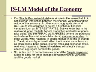
IS-LM Model of the Economy • Our Simple Keynesian Model was simple in the sense that it did not allow an interaction between the financial variables and the output of the economy. In other words, aggregate demand (C+I+G+X) was assumed to be not a function of financial variables such as INTEREST RATES. But we know that in the real world, good markets (where production and sales of goods take place) and the FINANCIAL MARKETS (where the purchase and sales of financial assets take place) are interdependent. In other words, what happens in goods market (in terms of change in Y and prices of goods) will affect the financial variables such as stock prices, bond prices, interest rates and exchange rates. And what happens to financial variables will affect Y through effect on aggregate demand for goods. • So, in this part of our lectures we extend the Simple Keynesian Model to allow for these linkages between financial variables and the goods market.
R (FINANCIAL) ASSETS MARKETS GOODS MARKET Y ECONOMY
In the IS-LM Model, we assume that the FINANCIAL SECTOR is made up of only 2 markets:MONEY MARKET and the BOND MARKET. (In the real world, we have additional types of asset markets such as STOCK MARKET, GOLD MARKET and others). • So in the IS-LM Model, the economy is made up of only 3 markets: • GOODS MARKET • MONEY MARKET • BOND MARKET
To analyze the equilibrium of the economy we need to focus on only two markets if we have 3 markets. Due to famous LAW of Economics called WALRAS’ LAW, if there are N markets in the economy, and if N-1 of them are in equilibrium, automatically Nth one must also be in equilibrium. So IS-LM Model analyses the equilibrium of the economy by focusing on the interaction between GOODS MARKET and the MONEY MARKET.
In what follows, we try to introduce the basic algebraic relationships of the goods market and then we try to do the same for the Money Market of the IS-LM Model (Note: We will explain later why this model is called IS-LM Model)
GOODS MARKET • Y= C + I + G + X Equilibrium condition for the good market • C= a + b(1-t)Y • I= e - dR d>0 • G = G • X=g-mY-nR m, n>0
As you can see the differences between the above model (of the good market) and the simple Keynesian model are the inclusion of R (Interest Rate) as an additional variable as a variable on the aggregate demand side of the economy through INVESTMENT and NET EXPORTS functions.
Eq. (3): I = e - dR implies that total investment spending is negatively affected by R. As R ↑I↓. (As the cost of borrowing from the banks ↑, naturally firms reduce their spending for new capital goods). e represents the amount of investment spending which depends on other factors such as business optimism about the future profits, technology and others.
X= g-mY-nR means that Net Exports (Trade Balance) is respectively affected both by Y and R. As Y ↑ we know that M (Imports) will ↑leading to a fall in X. HOW ABOUT the negative relationship between X and R? As R↑ X↓! WHY? • As R↑ interest rates on domestic bonds ↑, this makes domestic bonds more attractive than foreign bonds leading to increase in relative demand for domestic bonds by domestic and foreign portfolio investors. This leads to rising capital in flow to the domestic economy which raises the demand for domestic currency. • Higher demand for domestic currency leads to appreciation of the exchange rate making exports relatively more expensive and imports cheaper. And this leads to deterioration of trade balance: R ↑X↓.
So the key insight of the new Goods Market relationships (of the IS-LM model) is that FINANCIAL SECTOR affects the GOODS MARKET (REAL SECTOR of the economy) mainlythrough change in INTEREST RATES. • R↑ X↓ AD↓Y↓ • I↓
HOW ABOUT THE FINANCIAL SECTOR? • Earlier we said that to analyze the equilibrium of the financial sector, we need to focus only on one of the two markets. And here we analyze how the equilibrium in MONEY MARKET is maintained; • Just like any other market, Money market can be analyzed by focusing on the DEMAND and the SUPPLY sides of the market. • We first analyze the SUPPLY SIDE OF MONEY MARKET. • We assume that MONEY SUPPLY is exogenously given to the economy by the government. And government can change money supply (MS) any time and in any amount it wants to!
We define and measureMoney Supply using a “narrow measure” of money called M1. M1 is made up of currency in circulation + Demand deposits at the banks • So MS = C.C +D.D • C.C = Currency in Circulation • D.D =Demand Deposits (Checking Account)
NOTE: • In the real world, the actual process of bringing about a desired change in MS is not as easy as it looks. Government can change MS only indirectly through same policy instruments which primarily include: • OPEN MARKET OPERATIONS • DISCOUNT RATES • RESERVE RATIO
Read from your textbooks and other books how these policy instruments can be used to alter Ms!! • So, what is the message we should get from this description of Ms! • At a given point in time Ms is EXOGENOUSLY GIVEN to the Money Market and therefore to the ECONOMY by the policy makers. That is why Ms is a POLICY VARIABLE in our model. (Additional policy variables are G and t which affect the economy through their effects on Aggregate Demand!) • Government can change Ms for its policy purposes, leading to disequilibrium in the money market which, as we will see, cause changes in R. And changes in R will affect Y in the way described before.
To analyze the Money Market Equilibrium and what happens when this equilibrium is disturbed, we need to analyze DEMAND SIDE OF THE MONEY MARKET (as well) and then put theSupply and DemandSides together!
WHAT IS THE DEMAND FOR MONEY? • Md (DEMAND FOR MONEY) is simply the total amount of Money (in the form CC+DD) that households and the firms would like to hold at a given point in time.
WHY DO HOUSEHOLDS (consumers) AND THE FIRMS NEED or DEMAND MONEY? • There are three Motives for Demand for Money (which is actually a demand for an asset which does not earn an interest!)
MOTIVES FOR MONEY DEMAND • TRANSACTIONS MOTIVE • PRECAUTIONARY MOTIVE • SPECULATIVE MOTIVE
1. TRANSACTIONS MOTIVE • An important percentage of the existing demand for Money is the Transactions Demand for Money. We need to hold money in order to finance our transactions whose volume is a positive function of our income (Y) level. • So TRANSACTIONS DEMAND for MONEY increases as Y ↑!
2. PRECAUTIONARY MOTIVE • We hold money also for emergency purposes which is called precautionary motive. So some part of our Md is due to precautionary motive. And this PRECAUTIONARY DEMAND FOR MONEY also positively depends on the level of Y. As Y↑ Amount of money demanded ↑for precautionary reasons.
3. SPECULATIVE MOTIVE • Some people (and firms) may hold money for speculative reasons. In our model the other asset (in addition to money) is the BONDS. So speculation about the possible decline in Bond Prices in the future may make some people hold some money to take advantage of a possible decrease in bond prices. Remember that low bond prices automatically imply higher interest rates on these bonds. • So, if the present interest rates are perceived to be relatively low (meaning that the present bond prices are perceived to be high) speculators will increase their demand for money so as to be readily to buy bonds when the bond prices fall.
So, in our IS – LM Model SOME PART of the DEMAND for MONEY is the SPECULATIVE DEMAND for MONEY which is negatively affected by R! • As R (meaning Bond Price ), speculative Demand for money , • As Rspeculative demand for money.
The above 3 motives for Money Demand gave rise to the following mathematical relationship between Md (Money demand) and Y and R, • Md = Pf (Y, R)= P (kY- hR) k > 0 , h > 0 • Md=Amount of money Demanded depends on Y and R, and P ( Price level ) • As Y Md • As R Md
If P (price level for goods) , Md will automatically increase proportionately. • In the other words, given the values of k and h (which measure the sensitivity of Money demand to change in Y and R), we have a Real Demand for money; which is the demand for money measured in units of goods .If P (price of a unit of good) (amount of money in units of dollar) will increase in proportion to increase in P to keep the real demand for money same as before. • Read this from text books! • Md = P (kY - hR)
MONEY DEMAND FUNCTION! • So money demand (in nominal terms) depends on P,Y and R. • H1 P Md (proportionately) • Y Md (Increase depends on k) • R Md (decrease depends on h)
MONEY MARKET EQUILIBRIUM CONDITION • Ms = Md = P( kY- hR ) • Ms POLICY VARIABLE exogenously given by the government • P PREDETERMINED VARIABLE • P is given to the economy at the beginning of each period by the firms, that is why it is called Predetermined Variable! • It is determined in the beginning of each period .Firms can unexpectedly change P if there are some shocks to their costs of production! • Y and R are called ENDOGENOUS VARIABLES. (They will be determined by the interaction of the goods market and money market).
A PARTIAL EQUILIBRIUM ANALYSIS OF MONEY MARKET • (Partial means: We are not analyzing the money market in a general equilibrium frame work which includes goods market equilibrium and their interaction with each other. We will do this later when we fully develop graphical IS-LM Model.
Ms R E0 Shift Variables RE Md (P, Y) M (Quantity of Money) M0
Suppose government fixed Ms at M0. • So Ms curve is vertical curve at M0, (This means that in R has no effect on Ms. That’s why it is vertical! ) • Md curve is negatively sloped! • An ↑ ın R Md ↓ [due to lower speculative demand for money] • ↑ in P and ↑ in Y will shift the Md curve to the right. İn other words, Md will be higher (at each interest rate) when P↑ or Y↑! Higher P and higher Y increases the DEMAND for money)! • Given constant Ms at M0, and given P and Y, Money market will be in equilibrium at E0 which results in RE. To see what happens if Ms↑ (by the government) look at the following diagram!
R MS0 MS1 E0 A R0 E1 R1 Md(P0, Y0) M0 M1 M
When Ms ↑ from M0 to M1, Ms curve shifts to MS1, from MS0. At the initial equilibrium interst rate (R0) and given value of P0 and Y0, the means we have Excess Supply of money; M1>Md0(=M0) • M1: New Money Supply • Excess Supply of Money People attempt to get rid of excess money balance by buying the alternative asset (bonds) Demand for Bonds ↑ Bond Prices (Bp) ↑R↓ • As R↓ Md↑ and this process continues until R↓ by a sufficient amount which taken place at E1 (at which point Md=M1=MS).
So the key variable in adjustment of the money market to emergence of any excess supply or exess demand condition is the INTEREST RATE (R): • A-) If we have Ms>Md (Excess Money Supply) R↓ Md↑ Process continues until Ms=Md !!! • B-) If we have Ms<Md (Excess Demand for money) R↑Md↓The process continues until Ms=Md !!!
Notice that: • This adjustment mechanism is PARTIAL because is does not tell us what will happen to Y as R↑ or ↓. And if Y changes as a result of change in R, this will cause additional change in MONEY MARKET! IS-LM Model will tell us how this happens! • Suppose P↑ or Y↑ what happens?
R Ms E1 R1 A R0 E0 Md1(P1,Y0) Md0(P0,Y0) M0 MdA Y
If P↑ from P0 to P1 Md curve will shift from Md0 to Md1. So at the initial interest rate (R0), given a fixed Ms=M0, thiss will mean EXCESS DEMAND for money since the new level of Md will be given by point A (MdA). Excess Demand for money will make people to attempt to sell of their bonds and convert (at least some of them) to cash to bring their money balances to their desired level. As Bond Prices↓ R will ↑. Then increase in R will continue until R=R1and the money market is back in equilibrium at E1. • NOTE: Same analysis applies to changes in Y.
NOW WE ARE READY T INTRODUCE IS – LM MODEL OF THE ECONOMY: • IS represents the goods Market Equilibrium condition of the economy. • Originally when this model was developed for a closed economy with no public sector, goods market equilibrium condition was given by I = S! • LM represents the Money Market Equilibrium condition. • L Demand for money (Liquidity) • M Supply of Money • M = L
MATHEMATICAL STRUCTURE OF THE IS –LM MODEL • GOODS MARKET MONEY MARKET 1. Y = C + I + G + X 6. Ms = Md 2. C = a + b (1-t)Y 7. Ms = M 3. I = e – dR 8. Md = P (kY - hR) 4. G = G 5. X = g - mY - nR
In IS - LM model for the ECONOMY to be in EQUILIBRIUM we need to satisfy the eq. conditions for both the Money Market and the Goods Market! • In other words for the economy to be in equilibrium we require: • 1. Y = C + I + G + X and 6. Ms = Md at the same time. • So both GOODS M. and MONEY M. have to be in EQUILIBRIUM for the ECONOMY to be in equilibrium.
CLASSIFICATION OF VARIABLES IN IS - LM MODEL • EXOGENOUS VARIABLES a, e, g • So, same autonomous components of aggregate demand such as a, e, and g are called exogenous variables. • POLICY VARIABLES G, T, and Ms • Policy variables are also exogenous variables but we treat them separately. • ENDOGENOUS VARIABLES Y and R • PREDETERMINED VARIABLE: P • So, given the values of exogenous and policy variables (together with the values of the structural parameters of the model which are the coefficients like b, d, m, n, and h) and the value of the predetermined variable (P), the model determine the equilibrium value of Y and R (Endogenous variables). • EQUILIBRIUM VALUES OF Y AND R are those values of Y and R which will emerge when GOODS MARKET and the MONEY MARKET are in equilibrium, given the values of exogenous, policy, and predetermined variables.
R LM (Curve) E0 R0 IS (Curve) Y Y0 GRAPHICAL TOOLS OF IS - LM MODEL
IS CURVE • IS curve is a negatively sloped curve in (Y-R) space showing all the possible combinations of Y and R at which the Goods Market will be in equilibrium. The location of IS curve depends on the values of , G, t, a, g, e. • A given in G, a, g, or e will shift the IS curve to the right. A given will shift it to the left in a parallel fashion. (No change in slope). • A given t() will rotate the IS curve downward (upward) by changing its slope. (We will explain this later). • So along the IS curve, goods market is in equilibrium meaning that the values of (Y, R) are such that Y= AD= C+I+G+X at each point on the IS curve. • To understand why IS curve is negatively sloped look at the following example:
R B C RB (Excess Supply of goods) A RA D (Excess D for goods) (G, t, a, e, g) YC YA M
At A; YA=ADA (goods M. equilibrium). In other words, the values of (YA,RA) are such that the resulting values of CA, IA and XA (at these values of YA and RA), given the values of G, t, a, e, and g, will be such that YA = CA + IA + G + XA. • Suppose R from RA to RB. At point B, Y=YA, but R=RB!. • At B we will have EXCESS SUPPLY of goods in the goods market. Because R I X ADYA>ADB (Excess Supply of goods).
For the goods market to return back to equilibrium, we need Y=AD. • So at a HIGHER INTEREST RATE (such as RB), the only way to return back to equilibrium is to have LOWER Y (such as YC). • So starting from a point of equilibrium on the IS curve, an in R will require a in Y for the goods market to return back to equilibrium. • Similarly you can try and see yourself that a point such as D is a point of EXCESS DEMAND for goods market. • So in order to return back to equilibrium (after lowering interest rate from C to D (from RB to RA) we need to have an in Y. (Because: lower RAD (due to I and X) and this necessitates an in Y for equilibrium.
R RA A B IS1 IS0 (G, t, a, e, g) YA SHIFTS IN IS CURVE
If a, e, g, or G ↑(↓) this will lead to a parallel rightward (leftward) shift in IS curve. Why? After the ↑ in a or e or g or G at each interest rate we will have a HIGHER AD than before! (C + I + G + X = AD ↑) • So for the goods market to be in equilibrium we will need to have a HIGHER Y (than before). • If the value of t changes IS curve will rotate! (its slope will change!
R B RB A RA C RC RD D IS(t0) IS(t1) The effect of an in t on IS curve YA YD
The reason why a ∆ in t will rotate the IS curve in the way described above is as follows: • ∆ t affects AD through its effect on Yd (Disposable Income) and therefore through its effect on C which depends on Yd. • The above rotation suggests that at low-income levels such as YA, a given in t will require a in R given by the distance between B and A for the goods Market to return back to equilibrium. However if the same in t is taken place at a higher Y level (such as when Y=YD), we need to have a much bigger in R (from RC to RD) for the goods market to return back to equilibrium. On the other hand when Y=0, there is no ∆ in R required!
To understand the logic of this you have to focus on the effect of a given change in t on AD through its effect on C! • At lower Y levels, a given in t will reduce C by a lower amount simply because its effect on Yd (Disposable Income) will be lower. • Therefore the amount of excess supply that will result from a given in t will be smaller. And therefore with a relatively smaller in R AD can by enough amount to eliminate the relatively small excess supply. • However when Y is relatively high, same in t will lead to relatively larger in Yd and therefore relatively lower in C and in AD. And the elimination of this relatively bigger excess supply will require relatively bigger in R(such as a from RC to Rd!)
R LM (P0 M0) C RD D A RA B (Excess demand for Money) YA YB LM CURVE Excess supply of money