Sample Variability
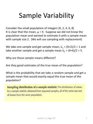
Sample Variability. Consider the small population of integers {0, 2, 4, 6, 8} It is clear that the mean, μ = 4. Suppose we did not know the population mean and wanted to estimate it with a sample mean with sample size 2. (We will use sampling with replacement)

Sample Variability
E N D
Presentation Transcript
Sample Variability Consider the small population of integers {0, 2, 4, 6, 8}It is clear that the mean, μ = 4. Suppose we did not know the population mean and wanted to estimate it with a sample mean with sample size 2. (We will use sampling with replacement) We take one sample and get sample mean, ū1 = (0+2)/2 = 1 and take another sample and get a sample mean ū2 = (4+6)/2 = 5. Why are these sample means different? Are they good estimates of the true mean of the population? What is the probability that we take a random sample and get a sample mean that would exactly equal the true mean of the population? Section 7.1, Page 137
Sampling Distribution Each of these samples has a sample mean, ū. These sample means respectively are as follows: P(ū = 1) = 2/25 = .08P(ū = 4) = 5/25 = .20 Section 7.1, Page 138
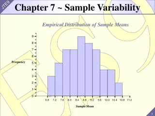
Sampling Distribution Shape is normal Mean of the sampling distribution = 4, the mean of the population Section 7.1, Page 138
Sampling Distributions and Central Limit Theorem Alternate notation: Sample sizes ≥ 30 will assure a normal distribution. Section 7.2, Page 141
Central Limit Theorem Section 7.2, Page 144
Central Limit Theorem Section 7.2, Page 145
Calculating Probabilities for the Mean Kindergarten children have heights that are approximately normally distributed about a mean of 39 inches and a standard deviation of 2 inches. A random sample of 25 is taken. What is the probability that the sample mean is between 38.5 and 40 inches? P(38.5 < sample mean <40) = NORMDIST 1 LOWER BOUND = 38.5 UPPER BOUND = 40 MEAN =39 ANSWER: 0.8881 Section 7.3, Page 147
Calculating Middle 90% Kindergarten children have heights that are approximately normally distributed about a mean of 39 inches and a standard deviation of 2 inches. A random sample of 25 is taken. Find the interval that includes the middle 90% of all sample means for the sample of kindergarteners. Sampling Distribution NORMDIST 2 AREA FROM LEFT = 0.05 MEAN = 39 ANSWER: 38.3421 NORMDIST 2 AREA FROM LEFT = .95 MEAN = 39 ANSWER: 39.6579 The interval (38.3 inches, 39.7 inches) contains the middle 90% of all sample means. If we choose a random sample, there is a 90% probability that it will be in the interval. Section 7.3, Page 147
Problems Problems, Page 149
Problems Problems, Page 150
Problems Problems, Page 151