PM 515 Behavioral Epidemiology Power Analysis
320 likes | 802 Vues
PM 515 Behavioral Epidemiology Power Analysis . Ping Sun, Ph.D. Jennifer Unger, Ph.D. Power Analysis. Introduction Understanding of Power analysis Power analysis for basic hypothesis test Power analysis in SAS Power Analysis for Two Leveled Trial Design

PM 515 Behavioral Epidemiology Power Analysis
E N D
Presentation Transcript
PM 515Behavioral EpidemiologyPower Analysis Ping Sun, Ph.D. Jennifer Unger, Ph.D.
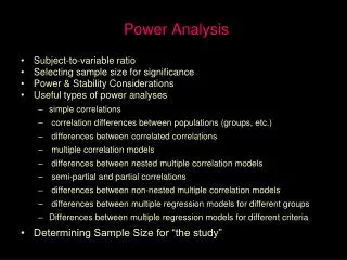
Power Analysis • Introduction • Understanding of Power analysis • Power analysis for basic hypothesis test • Power analysis in SAS • Power Analysis for Two Leveled Trial Design • Power analysis for cost effectiveness
Power Analysis: General Introduction • We run a regression with data from CSCS, and found that r=0.02, p=0.04. • We run another regression with data from TND CHS schools, r=0.06, p=0.15. • What does that mean?
Power Analysis: General Introduction • Should we report the r=0.02, p=0.04 finding from CSCS? • Yes, if r=0.02 means something of importance to public health. • With huge N in CSCS, a lot of significance would be showing up in analysis. • Should we report the r=0.06, p=0.15 finding? • even though it is important to public health, we do not have enough sample size to establish a significant conclusion ! • The understanding of p=0.15.
Decision Bar Power with Alpha, effect size, and N β α Blue distribution: estimated beta when the null hypothesis is true Red distribution: estimated beta when there is an effect
Power as critical consideration in study design • Three coupled parameters in power analysis (revisit slide #6 for more understanding) • Level of significance: alpha • Power increases when alpha is larger • Alpha for two-sided hypothesis test is only 50% for that for one-sided test. • Effect size • Power increases when effect size increases • Standard error of the estimation
Method to reduce standard error of the estimation • For linear regression, the variance of beta is proportional to the variance of the disturbance, and inversely proportional to the DoF of the disturbance • To increase the sample size • To reduce the variance of the disturbance • To increase the measurement precision in Y • To increase model fit
Power Calculation for Common Study Design • Equivalence of means across two groups • The significance of a correlation • Differences between correlation coefficients • Test of a Proportion equals to 50% • Differences between two proportions • Tests for Goodness of Fit and Contingency Tables • ANOVA • Multiple regressions
Equivalence of Means Across Two Groupspower for t test • Effect size: d = |m1-m2|/std • Std could be from either group when it is assumed to be the same across groups • D=0.2, 0.5, 0.8 are usually thought as small, medium, and large effect • Power will only be related to effect size, N, and alpha • When n is not the same: Naverage=2NaNb/(Na+Nb) • When std is not the same: std=sqrt(std12+std22)
The significance of a correlation • To convert it to a t test • T = r * sqrt(n-2) / sqrt(1-r2) • R = 0.1, 0.3, or 0.5 are usually considered small, medium, and large effect size
Differences between correlation coefficients • Power for (r=0.1 vs. r=0.3) is NOT the same as power for (r=0.4 vs. r=0.6) ! • Idea: to convert r to Z score • q = z1 – z2 • q=0.1, 0.3, and 0.5 are regarded as small, medium, and large effect size
Test of A Proportion Equals 50% • g = |p – 0.50| • G = 0.05, 0.15, and 0.25 are usually regarded as small, medium, and large effect sizes.
Differences Between Two Proportions • Φ = 2 arcsin[sqrt(p)] • h = |Φ1 – Φ2| • H = 0.20, 0.50, and 0.80 for small, medium, and large effect size
Tests for Goodness of Fit and Contingency Tables • Example of goodness of fit test: the % of ethnic groups are assumed to be 10%,40%, and 40% for AA, LATINO, and Non-Hispanic Whites. (example in notes area) • W=0.1, 0.3, and 0.5 for small, medium, and large effect • Power would be related to N, u, and W. The u is degree of freedom for the table. For a r by k contingency table, u=(r-1)*(k-1)
Power for 1-way ANOVA • f = σm / σ • σm = • f = 0.10, 0.25, and 0.40 for small, medium, and large effects • Power can be calculated from N, f, and u. u=k-1.
Power for interactions in Multi-factorial ANOVA • With two factors: Xij = mij – mi. – m.j + m. • σx = and f = σx /σ • With three-way interaction: • Xijk = mijk – mi – mj - mk – xij – xik - xjk + 2m • σx = and f = σx /σ • dof for interaction for 2-way, or three-way interaction would be (r-1)(c-1), or (r-1)*(c-1)*(h-1), accordingly.
Power for Multiple regressions • F test for overall model fitting • R2 for % variance explained by the model
Use SAS Proc Power to Conduct Power Analysis procpower; multreg model = random nfullpredictors = 7 ntestpredictors = 3 partialcorr = 0.35 ntotal = 100 power = .; run; procpower; multreg model = fixed nfullpredictors = 7 ntestpredictors = 3 rsquarefull = 0.9 rsquarediff = 0.1 ntotal = . power = 0.9; run; Proc Power design statistical model and test significance level (alpha) surmised effects and variability power sample size Run; proc power; onesamplemeans mean = 5 10 ntotal = 150 stddev = 30 50 power = .; plot x=n min=100 max=200; run;
Example: Proc Power for Logistic Regression proc power; logistic vardist("x1a") = normal(0, 2) vardist("x1b") = normal(0, 3) vardist("x2") = poisson(7) vardist("x3a") = ordinal((-5 0 5) : (.3 .4 .3)) vardist("x3b") = ordinal((-5 0 5) : (.4 .3 .3)) testpredictor = "x1a" "x1b" covariates = "x2" | "x3a" "x3b" responseprob = 0.15 testoddsratio = 1.75 covoddsratios = (2.1 1.4) ntotal = 100 power = .; run; To simulate two situations for the study variable To simulate two situations with different probability for the ordinal categorical variable
SAS Output: Power for Logistic Regressoin The POWER Procedure Likelihood ratio Chi-square test for one predictor Fixed Scenario Elements Method Shieh-O'Brien approximation Response Probability 0.15 Odds Ratio for Test Predictor 1.75 Covariate Odds Ratios 2.1 1.4 Total Sample Size 100 Alpha 0.05 Computed Power Test Total Test Pred N Index Pred -Covariates- Unit -Cov Units- Bins Power 1 x1a x2 x3a 1 1 1 300 0.931 2 x1a x2 x3b 1 1 1 300 0.927 3 x1b x2 x3a 1 1 1 300 0.999 4 x1b x2 x3b 1 1 1 300 0.999
Power for Multiple Regression The POWER Procedure Type III F Test in Multiple Regression Fixed Scenario Elements Method Exact Model Fixed X Number of Predictors in Full Model 7 Number of Test Predictors 3 R-square of Full Model 0.9 Difference in R-square 0.1 Nominal Power 0.9 Alpha 0.05 Computed N Total Actual N Power Total 0.903 20 procpower; multreg model = fixed nfullpredictors = 7 ntestpredictors = 3 rsquarefull = 0.9 rsquarediff = 0.1 ntotal = . power = 0.9; run;
Proc GLMPOWER for Power Analysisfor more complex situations Statement Components: • design (including subject profiles and their allocation weights) • statistical model • contrasts of class effects • significance level (alpha) • surmised response means for subject profiles (often called "cell means") • surmised variability • power • sample size
Proc GLMPower Example Mean Flower Height (in cm) by Variety and Exposure: data Exemplary; do Variety = 1 to 2; do Exposure = 1 to 3; input Height @@; output; end; end; datalines; 14 16 21 10 15 16 ; run; proc glmpower data=Exemplary; class Variety Exposure; model Height = Variety | Exposure; power stddev = 5 ntotal = 60 power = .; run;
Proc GLMPower Continued data Fluids2; input Altitude $ Fluid $ LacticAcidCellWgt; datalines; High Water 36.9 4 High EZD1 35.0 2 High EZD2 31.5 2 High LZ1 30 2 High LZ2 27.1 2 Low Water 34.3 6 Low EZD1 32.4 3 Low EZD2 28.9 3 Low LZ1 27 3 Low LZ2 24.7 3 ; run; proc glmpower data=Fluids2; class Altitude Fluid; model LacticAcid = Altitude Fluid; weight CellWgt; contrast "Water vs. others" Fluid -1 -1 -1 -1 4; contrast "EZD vs. LZ" Fluid 1 1 -1 -1 0; contrast "EZD1 vs. EZD2" Fluid 1 -1 0 0 0; contrast "LZ1 vs. LZ2" Fluid 0 0 1 -1 0; power nfractional stddev = 3.5 ncovariates = 1 corrxy = 0.2 0.3 0 alpha = 0.025 ntotal = . power = 0.9; run; Table 34.9: Mean Lactic Acid Buildup by Fluid and Altitude Table 34.10: Approximate Sample Size Allocation Weights
Power in Two-Leveled Random Effects Model • Randomization and treatment assignment conducted on group level • School, clinical site, etc. • Observation conducted on subject level • Two considerations: • Degree of freedom for effectiveness test • Intra-class correlation
Mathematical perspective Assume there is g schools in each condition, m students in each school and the within school variance of Var(y), The variance of the school mean would be: Var(y)/m The variance for the condition mean would be: Var(y) / (m*g) The intra-class correlation serves to reduce the variation among students in the same school so that the within school variance of the simplest school-randomized trial is: Varws(y) = Var(y) (1-ICC) = Var(y) - Varbs(y) The variance of the school mean would then be: (Varws(y) + Varbs(y) ) /m = Varws(y) / m + Varbs(y) ) = Var(y) (1-ICC) /m + Var(y) * ICC = [ Var(y) / m ] * [1-ICC+m*ICC] = [ Var(y) / m ] * [1 + (m-1) * ICC ] If school is the unit of analysis, the above formula would mean that the power would be equivalent to study a subject level hypothesis with m subjects, but with the variance expanded to [1 + (m-1) * ICC ] * Var(y). Or: it is the same as to study a subject level hypothesis with the same effect size, but need to expand the required N by a expansion factor [1 + (m-1) * ICC ].
An Excel file to help conduct the power analysis • ..\..\..\MODEL\clustered sampling\keiths clustered power.xls
Sample Size Needed for Moderation Effect Analysis (if standard error (se) for a main effect β is ‘x’, divide the whole sample equally into two sub-groups, the se for effects in each sub-group is ‘x*21/2’. The se for the moderating effect, which was the difference in effects between two sub-groups, is therefore ‘2*x’; Thus, if a simple size N is needed to reveal a main effect of size β, the sample size of 4*N is needed to reveal a moderating effect of equivalent effect size β. For two –level study with school and subject level, it means that 4 time of the number of schools are needed. As for only increase number of subjects in each school, or to increase both number of schools, and number of subjects, need to calculate from the basic formula of [ Var(y) / m ] * [1 + (m-1) * ICC ]
Maximize Power When Per Subject Cost Is Not Even: An Example Example: For a study of case-control design, total budget is $1000, $3 is needed for each case subject, $2 is needed for each control subject. To achieve the highest power to explore for a risk factor, how many case subjects and control subjects should we recruit? See sample.xls for solution.
