Understanding Hypergraphs and Dual Graphs in Acyclic Networks
This chapter delves into hypergraphs, dual graphs, and their applications in acyclic networks. It defines hypergraphs as sets of nodes and hyperedges, explaining how dual graphs represent hyperedges as nodes with shared vertices. The primal graph of a hypergraph is also detailed, highlighting the relationship between constraints and connectivity. The concept of acyclic networks is explored through the running intersection property, join graphs, and hypertrees. Additionally, the chapter discusses algorithms for solving acyclic networks, complexities involved, and recognition techniques, including both dual and primal approaches.

Understanding Hypergraphs and Dual Graphs in Acyclic Networks
E N D
Presentation Transcript
Tree Decomposition methodsChapter 9 ICS-275 Spring 2009
Graph concepts reviews:Hyper graphs and dual graphs • A hypergraph is H = (V,S) , V= {v_1,..,v_n} and a set of subsets Hyperegdes: S={S_1, ..., S_l }. • Dual graphs of a hypergaph: The nodes are the hyperedges and a pair of nodes is connected if they share vertices in V. The arc is labeled by the shared vertices. • A primal graph of a hypergraph H = (V,S) has $V$ as its nodes, and any two nodes are connected by an arc if they appear in the same hyperedge. • if all the constraints of a network R are binary, then its hypergraph is identical to its primal graph.
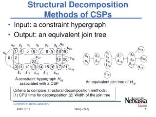
Acyclic Networks • The running intersection property (connectedness): An arc can be removed from the dual graph if the variables labeling the arcs are shared along an alternative path between the two endpoints. • Join graph: An arc subgraph of the dual graph that satisfies the connectedness property. • Join-tree: a join-graph with no cycles • Hypertree: A hypergraph whose dual graph has a join-tree. • Acyclic network: is one whose hypergraph is a hypertree.
Solving acyclic networks • Algorithm acyclic-solving applies a tree algorithm to the join-tree. It applies (a little more than) directional relational arc-consistency from leaves to root. • Complexity: acyclic-solving is O(r l log l) steps, where r is the number of constraints and l bounds the number of tuples in each constraint relation • (It assumes that join of two relations when one’s scope is a subset of the other can be done in linear time)
Example • Constraints are: • R_{ABC} = R_{AEF} = R_{CDE} = {(0,0,1) (0,1,0)(1,0,0)} • R_{ACE} = { (1,1,0) (0,1,1) (1,0,1) }. • d= (R_{ACE},R_{CDE},R_{AEF},R_{ABC}). • When processing R_{ABC}, its parent relation is R_{ACE}; • processing R_{AEF} we generate relation • processing R_{CDE} we generate: • R_{ACE} = \pi_{ACE} ( R_{ACE} x R_{CDE} ) = {(0,1,1)}. • A solution is generated by picking the only allowed tuple for R_{ACE}, A=0,C=1,E=1, extending it with a value for D that satisfies R_{CDE}, which is only D=0, and then similarly extending the assignment to F=0 and B=0, to satisfy R_{AEF} and R_{ABC}.
Recognizing acyclic networks • Dual-based recognition: • perform maximal spanning tree over the dual graph and check connectedness of the resulting tree. • Dual-acyclicity complexity is O(e^3) • Primal-based recognition: • Theorem (Maier 83): A hypergraph has a join-tree iff its primal graph is chordal and conformal. • A chordal primal graph is conformal relative to a constraint hypergraph iff there is a one-to-one mapping between maximal cliques and scopes of constraints.
Check cordality using max-cardinality ordering. Test conformality Create a join-tree: connect every clicque to an earlier clique sharing maximal number of variables Primal-based recognition
Tree-based clustering • Convert a constraint problem to an acyclic-one: group subset of constraints to clusters until we get an acyclic problem. • Hypertree embedding of a hypergraph H = (X,H) is a hypertree S = (X, S) s.t., for every h in H there is h_1 in S s.t. h is included in h_1. • This yield algorithm join-tree clustering • Hypertree partitioning of a hypergraph H = (X,H) is a hypertree S = (X, S) s.t., for every h in H there is h_1 in S s.t. h is included in h_1 and X is the union of scopes in h_1.
Join-tree clustering • Input: A constraint problem R =(X,D,C) and its primal graph G = (X,E). • Output: An equivalent acyclic constraint problem and its join-tree: T= (X,D, {C ‘}) • 1. Select an d = (x_1,...,x_n) • 2. Triangulation(create the induced graph along $d$ and call it G^*: ) • for j=n to 1 by -1 do • E E U {(i,k)| (i,j) in E,(k,j) in E } • 3. Create a join-tree of the induced graph G^*: • a. Identify all maximal cliques (each variable and its parents is a clique). • Let C_1,...,C_t be all such cliques, • b. Create a tree-structure T over the cliques: • Connect each C_{i} to a C_{j} (j < I) with whom it shares largest subset of variables. • 4. Place each input constraint in one clique containing its scope, and let • P_i be the constraint subproblem associated with C_i. • 5. Solve P_i and let {R'}_i $ be its set of solutions. • 6. Return C' = {R'}_1,..., {R'}_t the new set of constraints and their join-tree, T. • Theorem: join-tree clustering transforms a constraint network into an acyclic network
THEOREM 5 (complexity of JTC) join-tree clustering is O(r k^ (w*(d)+1)) time and O(nk^(w*(d)+1)) space, where k is the maximum domain size and w*(d) is the induced width of the ordered graph. The complexity of acyclic-solving is O(n w*(d) (log k) k^(w*(d)+1)) Complexity of JTC
Unifying tree-decompositions • Let R=<X,D,C> be a CSP problem. A tree decomposition for R is <T,,>, such that • T=(V,E) is a tree • associates a set of variables (v)X with each node v • associates a set of functions (v)C with each node v such that • 1. RiC, there is exactly one v such that Ri(v) and scope(Ri)(v). • 2. xX, the set {vV|x(v)} induces a connected subtree.
HyperTree Decomposition • Let R=<X,D,C> be CSP problem. A tree decomposition is <T,,>, such that • T=(V,E) is a tree • associates a set of variables (v)X with each node • associates a set of functions (v)C with each node such that • 1. RiC, there is exactly one v such that Ri(v) and scope(Ri)(v). • 1a. v, (v) scope((v)). • 2. xX, the set {vV|x(v)} induces a connected subtree. w (tree-width) = maxvV |(v)| hw (hypertree width) = maxvV | (v)| sep (max separator size) = max(u,v) |sep(u,v)|
Example of two join-trees again Tree decomposition hyperTree- decomposition
Cluster Tree Elimination • Cluster Tree Elimination (CTE) works by passing messages along a tree-decomposition • Basic idea: • Each node sends one message to each of its neighbors • Nodeu sends a message to its neighborvonly whenureceived messages from all its other neighbors
x1 m(u,v) v u x2 xn Constraint Propagation
A B C R(a), R(b,a), R(c,a,b) 1 A BC B B C D F R(d,b), R(f,c,d) 2 E C D BF B E F R(e,b,f) 3 F G EF E F G R(g,e,f) 4 Join-Tree Decomposition(Dechter and Pearl 1989) • Each function in a cluster • Satisfy running intersection property • Tree-width: number of variables in a cluster-1 • Equals induced-width
Cluster Tree Elimination A B C R(a), R(b,a), R(c,a,b) 1 project join BC B C D F R(d,b), R(f,c,d),h(1,2)(b,c) 2 sep(2,3)={B,F} elim(2,3)={C,D} BF B E F R(e,b,f), h(2,3)(b,f) 3 EF E F G R(g,e,f) 4
1 ABC A BC B 2 BCDF E C D BF F 3 BEF G EF 4 EFG CTE: Cluster Tree Elimination Time: O ( exp(w*+1 )) Space: O ( exp(sep)) Time: O(exp(hw)) (Gottlob et. Al., 2000)
Cluster Tree Elimination - properties • Correctness and completeness: Algorithm CTE is correct, i.e. it computes the exact joint probability of every single variable and the evidence. • Time complexity: O ( deg (n+N) d w*+1 ) • Space complexity: O ( N d sep) where deg = the maximum degree of a node n = number of variables (= number of CPTs) N = number of nodes in the tree decomposition d = the maximum domain size of a variable w* = the induced width sep = the separator size Time and space by hyperwidth only if hypertree decomposition: time and O(N t^w*) space,
Cluster-Tree Elimination (CTE) m(u,w) = sep(u,w) [j {m(vj,u)} (u)] (u) (u) ... m(v1,u) m(vi,u) m(v2,u)
Distributed relational arc-consistency example A The message that R2 sends to R1 is R1 updates its relation and domains and sends messages to neighbors B C D F G
A A A A AB AC A C AB A B B ABD BCF F D DFG Distributed Arc-Consistency DR-AC can be applied to the dual problem of any constraint network. b) Constraint network
1 A A 3 A 2 AB AC B A C B 5 4 ABD BCF 6 F D DFG DR-AC on a dual join-graph
1 A A 3 A 2 AB AC B A C B 5 4 ABD BCF 6 F D DFG Iteration 1 B 1 3
1 A A 3 A 2 AB AC B A C B 5 4 ABD BCF 6 F D DFG Iteration 1
B 1 1 A 3 A 3 A 2 AB AC B A C B 5 4 ABD BCF 6 F D DFG Iteration 2
1 A A 3 A 2 AB AC B A C B 5 4 ABD BCF 6 F D DFG Iteration 2
1 A A 3 A 2 AB AC B A C B 5 4 ABD BCF 6 F D DFG Iteration 3
1 A A 3 A 2 AB AC B A C B 5 4 ABD BCF 6 F D DFG Iteration 3
1 A A 3 A 2 AB AC B A C B 5 4 ABD BCF 6 F D DFG Iteration 4
1 A A 3 A 2 AB AC B A C B 5 4 ABD BCF 6 F D DFG Iteration 4
1 A A 3 A 2 AB AC B A C B 5 4 ABD BCF 6 F D DFG Iteration 5
1 A A 3 A 2 AB AC B A C B 5 4 ABD BCF 6 F D DFG Iteration 5
Adaptive-consistency as tree-decomposition • Adaptive consistency is a message-passing along a bucket-tree • Bucket trees: each bucket is a node and it is connected to a bucket to which its message is sent. • The variables are the clicue of the triangulated graph • The funcions are those placed in the initial partition
E D || RDCB C || RACB || RAB B RA A A || RDB D C B E Bucket EliminationAdaptive Consistency(Dechter and Pearl, 1987) RCBE || RDBE , || RE
Adaptive-Tree-Consistency as tree-decomposition • Adaptive consistency is a message-passing along a bucket-tree • Bucket trees: each bucket is a node and it is connected to a bucket to which its message is sent. • Theorem: A bucket-tree is a tree-decomposition Therefore, CTE adds a bottom-up message passing to bucket-elimination. • The complexity of ATC is O(r deg k^(w*+1))
A C A ABC C A A ABC C BC ABCDE A ABCDE BCE A AB BC C AB BC DE CE CDE B ABDE BCE ABDE BCE BE CDEF CDEF C C DE CE FGH DE CE E C D F F F GH CDEF CDEF GHI GI H FGI GHIJ FGHI GHIJ F FGH H F H FGH H F F FG GH H G F GH more accuracy GI GHIJ FGI GI FGI GHIJ less complexity Join-Graphs and Iterative Join-graph propagation (IJGP)