Layout
Layout. Introduction General remarks Model development and validation The surface energy budget The surface water budget Link with CO2 budget Soil heat transfer Soil water transfer Snow Initial conditions Conclusions and a look ahead. H. LE. Day. D. Night. G.

Layout
E N D
Presentation Transcript
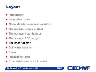
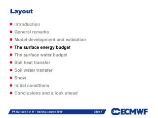
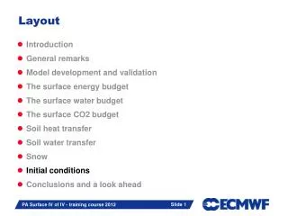
PA Surface II of IV - training course 2013 Layout • Introduction • General remarks • Model development and validation • The surface energy budget • The surface water budget • Link with CO2 budget • Soil heat transfer • Soil water transfer • Snow • Initial conditions • Conclusions and a look ahead
PA Surface II of IV - training course 2013 H LE Day D Night G Thermal budget of a ground layer at the surface
PA Surface II of IV - training course 2013 Dry Fir canopy Barley field Energy budget: Summer examples Arya, 1988
PA Surface II of IV - training course 2013 Surface albedo Surface emissivity Skin temperature The surface radiation • In some cases (snow, sea ice, dense canopies) the impinging solar radiations penetrates the “ground” layer and is absorbed at a variable depth. In those cases, an extinction coefficient is needed. Arya, 1988
PA Surface II of IV - training course 2013 Sensible heat flux specify the surface Evaporation Ground heat flux The other terms
PA Surface II of IV - training course 2013 Recap: The surface energy equation • Equation for • For: • a thin soil layer at the top • G (Ts,Tsk) is known, or parameterized or G << Rn we have a non-linear equation defining the skin temperature
PA Surface II of IV - training course 2013 Land Sea and ice High vegetation Open sea / unfrozen lakes Low vegetation Sea ice / frozen lakes High vegetation with snow beneath Snow on low vegetation Bare ground Interception layer Tiles
PA Surface II of IV - training course 2013 Fields ERA15 TESSEL Vegetation Fraction Fraction of low Fraction of high Vegetation type Global constant (grass) Dominant low type Dominant high type Albedo Annual Monthly LAI rsmin Global constants Annual, Dependent on vegetation type Root depth Root profile 1 m Global constant Annual, Dependent on vegetation type TESSEL geographic characteristics
PA Surface II of IV - training course 2013 High vegetation fraction at T511 (now at T1279) Aggregated from GLCC 1km
PA Surface II of IV - training course 2013 Low vegetation fraction at T511 (now at T1279) Aggregated from GLCC 1km
PA Surface II of IV - training course 2013 High vegetation type at T511 (now at T1279) Aggregated from GLCC 1km
PA Surface II of IV - training course 2013 Low vegetation type at T511 (now at T1279) Aggregated from GLCC 1km
PA Surface II of IV - training course 2013 Layout • Introduction • General remarks • Model development and validation • The surface energy budget • The surface water budget • Link with CO2 budget • Soil heat transfer • Soil water transfer • Snow • Initial conditions • Conclusions and a look ahead
PA Surface II of IV - training course 2013 Snow Lake Dry vegetation Wet vegetation Bare ground Evaporation: Idealized surfaces
PA Surface II of IV - training course 2013 • Evaporation efficiency • Ratio of evaporation to potential evaporation • Bucket model Budyko 1963, 1974 Manabe 1969 1 0 Potential evaporation, bucket model • Potential evaporation • The evaporation of a large uniform surface, sufficiently moist or wet (the air in contact to it is fully saturated)
PA Surface II of IV - training course 2013 A general, algebraic formulation • Two limit behaviours • Bare soil: Evaporation dependent on soil water (and trapped water vapor) in a top shallow layer of soil (~ 20 mm). • Vegetated surfaces: Evaporation controlled by a canopy resistance, dependent on shortwave radiation, water on the root zone (~ 1-5 m deep) and other physical/physiological effects.
PA Surface II of IV - training course 2013 Bare ground evaporation • Soil (bare ground) evaporation is due to: • Molecular diffusion from the water in the pores of the soil matrix up to the interface soil atmosphere (z0q) • Laminar and turbulent diffusion in the air between z0q and screen level height • All methods are sensitive to the water in the first few cm of the soil (where the water vapour gradient is large). In very dry conditions, water vapour inside the soil becomes dominant
PA Surface II of IV - training course 2013 TESSEL bare ground evaporation
PA Surface II of IV - training course 2013 New bare soil evaporation(Balsamo et al. 2011, Albergel et al. 2012) • SOIL EvaporationBalsamo et al. (2011) based on Mahfoufand Noilhan (1991) ut_2129 ####2010### R = 0.583 Bias = 0.005 RMSD= 0.068 ####2011### R = 0.906 Bias = 0.033 RMSD= 0.056 ut_2130 ####2010### R = 0.685 Bias = -0.036 RMSD= 0.064 ####2011### R = 0.812 Bias = -0.037 RMSD= 0.052 f2(w1) The introduction of bare groundevaporation revision (green-line) is quiteeffectivein reducing the soil moisture below the wilting point in non-vegetated area (upper panel of figure above, at79% bare ground, SCAN site in Utah). Rc=Rsoil f2(w1) ICOS Annual meeting, Bruxelles 1/6/2011 - G. Balsamo
PA Surface II of IV - training course 2013 Land Sea and ice High vegetation Open sea / unfrozen lakes Low vegetation Sea ice / frozen lakes High vegetation with snow beneath Snow on low vegetation Bare ground Interception layer Tiles
PA Surface II of IV - training course 2013 Transpiration: The big leaf approximation • Sensible heat (H), the resistance formulation • Evaporation (E), the resistance formulation (the big leaf approximation, Deardorff 1978, Monteith 1965)
PA Surface II of IV - training course 2013 Some plant science • rs, the stomatal resistance of a single leaf. Physiological control of water loss by the vegetation. Stomata (valve-like openings) regulate the outflow of water vapour (assumed to be saturated in the stomata cells) and the intake of CO2 from photosynthesis. The energy required for the opening is provided by radiation (Photosynthetically Active Radiation, PAR). In many environments the system appears to be operate in such a way to maximize the CO2 intake for a minimum water vapour loss. When soil moisture is scarce the stomatal apertures close to prevent wilt and dessication of the plant.
PA Surface II of IV - training course 2013 Jarvis approach(1) Dickinson et al 1991
PA Surface II of IV - training course 2013 Jarvis approach(2) Shuttleworth 1993
PA Surface II of IV - training course 2013 TESSEL transpiration
PA Surface II of IV - training course 2013 TESSEL root profile
PA Surface II of IV - training course 2013 TESSEL evaporation: shaded snow • Evaporation is the sum of the contribution of the snow underneath (with an additional resistance, ra,s ,to simulate the lower within canopy wind speed) and the exposed canopy. The former is dominant in early spring (frozen soils) and the latter is dominant in late spring.
PA Surface II of IV - training course 2013 Interception (1) • Interception layer represents the water collected by interception of precipitation and dew deposition on the canopy leaves (and stems) • Interception (I) is the amount of precipitation (P) collected by the interception layer and available for “direct” (potential) evaporation. I/P ranges over 0.15-0.30 in the tropics and 0.25-0.50 in mid-latitudes. • Leaf Area Index (LAI) is (projected area of leaf surface)/(surface area) 0.1 < LAI < 6 • Two issues • Size of the reservoir • Cl, fraction of a gridbox covered by the interception layer • T=P-I; Throughfall (T) is precipitation minus interception
PA Surface II of IV - training course 2013 Interception: Canopy water budget
PA Surface II of IV - training course 2013 TESSEL: interception • Interception layer for rainfall and dew deposition
PA Surface II of IV - training course 2013 Example: Deep tropics interception ARME, 1983-1985, Amazon forest Accumulated water fluxes Interception Evaporation Interception Viterbo and Beljaars 1995
PA Surface II of IV - training course 2013 Layout • Introduction • General remarks • Model development and validation • The surface energy budget • The surface water budget • Link with CO2 budget • Soil heat transfer • Soil water transfer • Snow • Initial conditions • Conclusions and a look ahead
PA Surface II of IV - training course 2013 (Calvet et al. 2005) Towards an increased vegetation complexity “old/standard” LSMs “new/photosynthesis- based” LSMs Slide 33
PA Surface II of IV - training course 2013 Jarvis-type Based parameterisation and LAI impact on screen level temperature For vegetated area the evapotranspiration is parameterized as: Where the canopy resistance rc is defined following Jarvis(1976) as: Where rs,min is the minimum stomatal resistance, LAI is the leaf area index and f1 , f2 , f3 are respectively function of the downward shortwave radiation Rs, soil moisture and vapour deficit Da If LAI then rc and E so T2m If LAI then rc and E so T2m
PA Surface II of IV - training course 2013 Previous Operational Yearly LAI map MODIS LAI (Myneni et al., 2002) Obtained by the inversion of a 3D radiative transfer model which compute the LAI and FPAR based on the biome type and an atmospherically corrected surface reflectance thanks to a look-up-table Slide 35 derived 8years (2000-2008) climatological time serie (Jarlan et al. 2008)
PA Surface II of IV - training course 2013 Impact of the usage of the MODIS based monthly LAI climatology on the 2m Temperature Sensitivity (warming) Impact (error reduction) Results from forecast experiments using MODIS LAI relative to the fixed LAI case for MAM at FC+36 (valid 12UTC), 2m temperature [K]
PA Surface II of IV - training course 2013 Land carbon/photosynthesis-based parameterisation (CTESSEL) RMetS National meeting 18 Jan 2012. S. Boussetta
PA Surface II of IV - training course 2013 Q10 T [oC] Soil Respiration parameterization(1) The Berry and Raison (1982) Q10 approach) Q10 represents the proportional increase of a parameter for a 10 degree increase in temperature (Berry and Raison, 1982) Including a temeperature dependency on the Q10 parameter (McGuire et al., 1992) Including a snow attenuation effect on the soil CO2 emission
PA Surface II of IV - training course 2013 Soil Respiration parametrization (2) Example of NEE (micro moles /m2/s) predicted over the site Fi-Hyy taking the cold process into account (right) and previous simulation (left) by CTESSEL (black line) and observed (red dots) Feedback from the atmosphere can contribute to improve the physical understanding and adjust the contribution from the surface
Jarvis Vs photosynthesis-based evapotranspiration PA Surface II of IV - training course 2013 CTESSEL HTESSEL H Surface sensible heat flux (W/m2) compared with flux-tower observations over Fr-LBr for HTESSEL (left panel) and CTESSEL (right panel) LE Surface laten heat flux (W/m2) compared with flux-tower observations over Fr-LBr for HTESSEL (left panel) and CTESSEL (right panel). • CTESSEL improves the LE/H simulations (Photosynthesis-based vs Jarvis approach).
PA Surface II of IV - training course 2013 CO2 exchanges as part of the daily forecasts Example of Average 10 days forecasted NEE from the 1st of June 2011 extracted from the pre-operational run (e-suites) [micromoles/m2/s] – Operational from November 2011
PA Surface II of IV - training course 2013 Impact of climate anomalies on CO2 flux: The summer 2003 2m temp precipitation Observedanomaly NEE July 2004 shown for comparison CTESSELmodelanomaly • Summer 2003 heat-wave/drought hitting western Europe. The effect on NEE was to turn land into a CO2 source due to vegetation stress conditions, consistently with findings of P. Ciais et al. (2005, Nature)
PA Surface II of IV - training course 2013 The 2010 Russian summer heat wave NEE anomaly LAI anomaly H anomaly Impact on 2m T and Rh forecast LE anomaly