Lecture 8 Chapter 5: CPU Scheduling
Lecture 8 Chapter 5: CPU Scheduling. Chapter 5: CPU Scheduling. Basic Concepts Scheduling Criteria Scheduling Algorithms Thread Scheduling Multiple-Processor Scheduling Operating Systems Examples Algorithm Evaluation. Objectives.

Lecture 8 Chapter 5: CPU Scheduling
E N D
Presentation Transcript
Chapter 5: CPU Scheduling • Basic Concepts • Scheduling Criteria • Scheduling Algorithms • Thread Scheduling • Multiple-Processor Scheduling • Operating Systems Examples • Algorithm Evaluation
Objectives • To introduce CPU scheduling, which is the basis for multiprogrammed operating systems • To describe various CPU-scheduling algorithms • To discuss evaluation criteria for selecting a CPU-scheduling algorithm for a particular system
Basic Concepts • Maximum CPU utilization obtained with multiprogramming • CPU–I/O Burst Cycle: Process execution consists of a cycle of CPU execution and I/O wait • Alternating Sequence of CPU And I/O Bursts
CPU Scheduler • Selects from among the processes in memory that are ready to execute, and allocates the CPU to one of them • CPU scheduling decisions may take place when a process: 1. Switches from running to waiting state 2. Switches from running to ready state 3. Switches from waiting to ready • Terminates • Scheduling under 1 and 4 is nonpreemptive • Processes keep CPU until it releases either by terminating or I/O wait. • All other scheduling is preemptive • Interrupts
Dispatcher • Dispatcher module gives control of the CPU to the process selected by the short-term scheduler; this involves: • switching context • switching to user mode • jumping to the proper location in the user program to restart that program • Dispatch latency – time it takes for the dispatcher to stop one process and start another running
Scheduling Criteria • CPU utilization – keep the CPU as busy as possible • Typically between 40% to 90% • Throughput – # of processes that complete their execution per time unit • Depends on the length of process • Turnaround time – amount of time to execute a particular process • Sum of wait for memory, ready queue, execution, and I/O. • Waiting time – amount of time a process has been waiting in the ready queue • Sum of wait in ready queue • Response time – amount of time it takes from when a request was submitted until the first response is produced, not output • for time-sharing environment
Scheduling Algorithm Optimization Criteria • Max CPU utilization • Max throughput • Min turnaround time • Min waiting time • Min response time • In most cases, systems optimize average measure • It is important to minimize variance • Users prefer predictable response time to faster system with high variances.
P1 P2 P3 0 24 27 30 First-Come, First-Served (FCFS) Scheduling ProcessBurst Time P1 24 P2 3 P3 3 • Suppose that the processes arrive in the order: P1 , P2 , P3 The Gantt Chart for the schedule is: • Waiting time for P1 = 0; P2 = 24; P3 = 27 • Average waiting time: (0 + 24 + 27)/3 = 17
P2 P3 P1 0 3 6 30 FCFS Scheduling (Cont) Suppose that the processes arrive in the order P2 , P3 , P1 • The Gantt chart for the schedule is: • Waiting time for P1 = 6;P2 = 0; P3 = 3 • Average waiting time: (6 + 0 + 3)/3 = 3 • Much better than previous case • Nonpreemtive • Convoy effect short process behind long process
Shortest-Job-First (SJF) Scheduling • Associate with each process the length of its next CPU burst. • Use these lengths to schedule the process with the shortest time • shortest-next-CPU-burst • SJF is optimal • Gives minimum average waiting time for a given set of processes • The difficulty is knowing the length of the next CPU request • SFJ scheduling is preferred for long-term scheduling
P3 P2 P4 P1 3 9 16 24 0 Example of SJF Process Arrival TimeBurst Time P1 0.0 6 P2 2.0 8 P3 4.0 7 P4 5.0 3 • SJF scheduling chart • Average waiting time = (3 + 16 + 9 + 0) / 4 = 7
Determining Length of Next CPU Burst • Can only estimate the length • Can be done by using the length of previous CPU bursts • using exponential averaging
Examples of Exponential Averaging • =0 • n+1 = n • Recent history does not count • =1 • n+1 = tn • Only the actual last CPU burst counts • If we expand the formula, we get: n+1 = tn+(1 - ) tn-1+ … +(1 - )j tn-j+ … +(1 - )n +1 0 • Since both and (1 - ) are less than or equal to 1, each successive term has less weight than its predecessor
Priority Scheduling • A priority number (integer) is associated with each process • The CPU is allocated to the process with the highest priority (smallest integer highest priority) • Preemptive • Nonpreemptive • SJF is a priority scheduling where priority is the predicted next CPU burst time • Problem Starvation • low priority processes may never execute • Solution Aging • as time progresses increase the priority of the process