Download
1 / 12
120 likes | 256 Vues
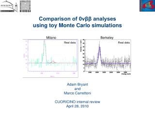
Comparison of 0νββ analyses using toy Monte Carlo simulations. Milano. Berkeley. Real data. Real data. Adam Bryant and Marco Carrettoni CUORICINO internal review April 28, 2010. Introduction.

E N D
Comparison of 0νββ analysesusing toy Monte Carlo simulations Milano Berkeley Real data Real data • Adam Bryant • and • Marco Carrettoni • CUORICINO internal review • April 28, 2010
Introduction • We have compared the Milano and Berkeley fitting and limit methods on toy Monte Carlo simulations. • Our goals are to compare the sensitivities of the two methods and to check for bias, especially when the hypothesis of equal background rates for crystals of the same type is not true. The Berkeley method assumes that this hypothesis is valid within statistical errors. • We performed three rounds of simulations (to be described). In each round, we simulated 1000 CUORICINO-like experiments with Γ = 0. • We analyzed each set of simulated data with both the Milano and Berkeley codes. • We used the same set of live times and resolutions for both analyses. • The results shown here for the Milano analysis were obtained using the sum-of-Gaussians response function. Similar results were obtained using the single-Gaussian response function, except that the errors were larger in that case.
Simulation round 1 setup • 1000 simulated experiments • CUORICINO exposures for each channel and data set • CUORICINO resolutions for each channel and data set • Γ = 0 • Equal background rates for crystals of the same type • Rates set equal to the average measured rates [counts / (keV kg y)]: • rbkg = 0.161 (big), rbkg = 0.163 (small), rbkg = 0.47 (enriched) • Equal 60Co rates for crystals of the same type • Rates set equal to the average measured rates [counts / (kg y)]: • r60Co = 3.1 (big), r60Co = 2.9 (small), r60Co = 0 (enriched) • Allows us to compare the sensitivities of the two methods when the hypotheses of the Berkeley fit are satisfied.
Simulation round 2 setup • 1000 simulated experiments • CUORICINO exposures for each channel and data set • CUORICINO resolutions for each channel and data set • Γ = 0 • Randomized background rates and 60Co rates for each channel • Drawn from a Gaussian distribution with mean equal to the average rate for the type of crystal and sigma equal to 20% of the average rate • rbkg ~ Gaussian(μ = 0.161, σ = 0.2 × 0.161) for big crystals • rbkg ~ Gaussian(μ = 0.163, σ = 0.2 × 0.163) for small crystals • rbkg ~ Gaussian(μ = 0.47, σ = 0.2 × 0.47) for enriched crystals • r60Co ~ Gaussian(μ = 3.1, σ = 0.2 × 3.1) for big crystals • r60Co ~ Gaussian(μ = 2.9, σ = 0.2 × 2.9) for small crystals • r60Co = 0 for enriched crystals • Different background rates for each simulated experiment • Allows us to check for bias in the Berkeley method when the hypothesis of equal rates is violated by an amount within the error bars on the CUORICINO data.
Simulation round 3 setup • 1000 simulated experiments • CUORICINO exposures for each channel and data set • CUORICINO resolutions for each channel and data set • Γ = 0 • Randomized background rates and 60Co rates for each channel • Drawn from uniform distributions: • rbkg ~ Uniform(0.1, 0.3) for big and small crystals • rbkg ~ Uniform(0.3, 0.7) for enriched crystals • r60Co ~ Uniform(2, 6) for all crystals • Different background rates for each simulated experiment • Allows us to check for bias in the Berkeley method with a more extreme violation of the hypothesis of equal rates. 9
Conclusion • There is a close correlation between the results of the two methods in all three rounds of simulations. • The Berkeley method has slightly smaller errors (by ~4%). However, for this comparison, the Milano method was not optimized as it is for CUORICINO by omitting channels and data sets with poor resolutions. • Both methods are unbiased even when the background rates vary by channel.