Download
1 / 73
780 likes | 1.24k Vues
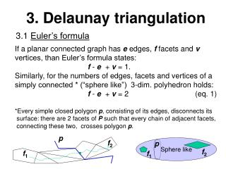
Delaunay Triangulation and Tetrahedrilization. Marc van Kreveld Slides DDM. Triangulations and their quality. When going from points on a surface to triangles representing that surface, there are many ways to form the triangles Some ways are better than others.

E N D
Delaunay Triangulation and Tetrahedrilization Marc van Kreveld Slides DDM
Triangulations and their quality • When going from points on a surface to triangles representing that surface, there are many ways to form the triangles • Some ways are better than others
Triangulations and their quality • This is not just true visually, but also when the triangulation is the interpolator for a terrain with elevation measurements
Triangulations and their quality • Triangulations are good if they • do not have long edges • do not have triangles with both short and long edges • do not have triangles with very small angles • do not have triangles with obtuse angles • do not have vertices with high degree • …
Voronoi diagrams • For a set of points (sites), the Voronoi diagram is the subdivision of the plane (space) with faces where exactly one of the sites is closest, among all sites
Voronoi diagrams • Voronoi vertices “often” have degree 3, but it can be much larger • Voronoi edges can be bounded or unbounded Voronoi edge Voronoi vertex
Voronoi diagrams • With n point sites, there are < 2nVoronoi vertices and < 3nVoronoi edges Voronoi edge Voronoi vertex
Voronoi diagrams • The average number of edges bounding a Voronoi cell is six (or slightly less), but a single cell could be bounded by up to n – 1 edges Voronoi edge Voronoi vertex
Voronoi diagrams • Voronoi diagrams have the empty circle property for every Voronoi vertex and Voronoi edge
Voronoi diagrams • Efficient algorithms exist to construct 2D Voronoi diagrams of n point sites, namely O(n log n) time algorithms (as fast as sorting! [mergesort, quicksort])
Voronoi diagrams • 3D Voronoi diagrams with n point sites can have up to (n2) Voronoi vertices (0D), Voronoi edges (1D), and Voronoi facets (2D) but of course just n cells (3D) • The descriptive complexity can be anything between linear and quadratic in n
Voronoi diagrams • 3D Voronoi diagrams with n point sites often have linearly many Voronoivertices (0D), Voronoi edges (1D), and Voronoi facets (2D)
Delaunay triangulation • For a set of points in the plane, suppose we compute its Voronoi diagram and use it to make an embedded planar graph G as follows: • all points are vertices of the graph G • for all points whose Voronoi cells share a Voronoi edge, we have an edge in G • faces of G are implied by the vertices and edges of G
Delaunay triangulation • all points are vertices of the graph G • edges in G correspond to edge-adjacent Voronoi cells • faces of G are implied by the vertices and edges of G
Delaunay triangulation • all points are vertices of the graph G • edges in G correspond to edge-adjacent Voronoi cells • faces of G are implied by the vertices and edges of G
Delaunay triangulation • This graph is called the Delaunay graph • Notice that an edge of the Delaunay graph does not necessarily intersect the corresponding Voronoi edge
Delaunay triangulation • The Delaunay graph is a triangulation of the original points if and only if all Voronoi vertices have degree 3 there is no circle through more than 3 sites and with no sites inside
Delaunay triangulation • Any (planar) completion of the Delaunay graph to a triangulation is a Delaunay triangulation of the original points
Delaunay triangulation • The empty-circle property for Voronoi diagrams transfers to Delaunay triangulations • for each triangle, its circumcirclecontains no other pointsfrom the set inside • for each edge, a circleexists through itsendpoints that hasno other points of theset inside
Delaunay triangulation • A Delaunay triangulation of n points has at least n – 2 and at most 2n – 5 triangles (Delaunay triangles) • A Delaunay triangulation of n points has at least 2n – 3 and at most 3n – 6 edges (Delaunay edges) • The empty-circle property is “if and only if”: if three points have a circumcircle with no points inside or other points on the boundary, then they make a Delaunay triangle(a similar statement holds for edges)
Delaunay triangulation • When a Delaunay graph is not a triangulation, the non-triangular faces have all vertices on a circle
Delaunay triangulation • When we know four Delaunay edges that form an empty convex quadrilateral, we will have one of the two diagonals as a Delaunay edge • The circumcircles of the triangles of one choice will contain the fourth points, but not for the other choice
Delaunay triangulation • The Delaunay triangulation maximizes the smallest occurring angle, over all triangulations of the point set • In other words, any other triangulation will have a smaller (or the same) smallest angle
Delaunay triangulation • The Delaunay triangulation often connects points close together, e.g., every point is connected to its nearest neighbor • But it does not minimize total edge length
Delaunay triangulation • In a triangulation, when two triangles form a convex quadrilateral, their shared edge can be replaced by one other edge • This is called an edge flip flip
Computing the Delaunay triangulation • Approach: insert points one-by-one, and restore the Delaunay triangulation after every insertion • Locate the triangle t con-taining the next point p • Connect p to t’s vertices • Restore the Delaunay triangulation by flipping non-Delaunay edges p t
Computing the Delaunay triangulation • Locate: Recall that we store triangulations in some convenient structure (triangle-neighbor structure, half-edge structure) • From any access point (triangle, half-edge), walkalong a straight line to thelocation of the p, finding the triangle t containing p • The details of the walk depend on the mesh structure used p
Computing the Delaunay triangulation • Connect: Make edges from p to t’s vertices; this replaces t by three new triangles • Adapt the mesh representationstructure accordinglyClaim: These three new edges are Delaunay p
Computing the Delaunay triangulation • Proof of claim: • Triangle t was Delaunay before the insertion of p, so there was an empty circle C through its vertices C v p t
Computing the Delaunay triangulation • Proof of claim: • Triangle t was Delaunay before the insertion of p, so there was an empty circle C through its vertices • Consider the edge between p andany vertex v of t, there is always acircle through p and vcompletely inside C (grow a small circle fromv tangent to C at v, until it hits p) C v p t
Computing the Delaunay triangulation • Proof of claim: • Triangle t was Delaunay before the insertion of p, so there was an empty circle C through its vertices • Consider the edge between p andany vertex v of t, there is always acircle through p and vcompletely inside C (grow a small circle fromv tangent to C at v, until it hits p) • Since v and p have an empty circle,they define a Delaunay edge C v p t
Computing the Delaunay triangulation • Restore: The three new edges are always Delaunay, but the three new triangles need not be … Delaunay p p maybe not Delaunay
Computing the Delaunay triangulation • In the picture: triangle qrs had an empty circle C(q,r,s) before the insertion of p, but maybe p lies inside now test p C(q,r,s), and if so, edge-flip qr to ps Delaunay q q C(q,r,s) p p s s r r maybe not Delaunay
Computing the Delaunay triangulation • If flipped, the edges pq, pr, and also ps must be Delaunay, but maybe pqs and prs are not Delaunay triangles … recurse on them, using the triangles opposite qs and rs Delaunay Delaunay q q p p s s r r maybe not Delaunay maybe not Delaunay
Computing the Delaunay triangulation • Code for recursive flipping (restore algorithm): TestFlipEdge (p, qr) Let s p be the third point of the triangle incident to qr ifp is inside C(q,r,s) { flip: delete qr and insert ps in the triangulation TestFlipEdge(p, qs) TestFlipEdge(p, sr) }
Computing the Delaunay triangulation • Comments: • The edge flip must be done in our triangle-mesh representation structure (triangle-neighbor, half-edge, …) • With suitable triangle-mesh structure, a flip takes O(1) time (with an indexed mesh, a flip takes O(n) time) • Every edge flip connects p to an extra vertex on the average, about 3 flips are needed • The main geometric test is the so-called in-circletest: does a point p lie inside the circle defined by three points q,r,s?
The in-circle test • The in-circletest: does a point p lie inside the circle defined by three points q,r,s? (1) The bad way: • Compute the bisectors of q,r and r,s • Intersect them to get the center c of C(q,r,s) • Compute dist(c,p) and dist(c,q) (the radius of C(q,r,s)); if the former is smaller, then p lies inside C(q,r,s)
The in-circle test • The in-circletest: does a point p lie inside the circle defined by three points q,r,s? (2) The good way: • Compute the plane through (qx, qy, qx2+ qy2), (rx, ry, rx2+ ry2), and (sx, sy, sx2+ sy2) • Test whether the point (px, py, px2+ py2) lies above or below this plane: below p is inside; above p is outside
The in-circle test • The in-circletest: does a point p lie inside the circle defined by three points q,r,s? (2) The good way: • Compute the plane through (qx, qy, qx2+ qy2), (rx, ry, rx2+ ry2), and (sx, sy, sx2+ sy2) • Test whether the point (px, py, px2+ py2) lies above or below this plane • This is equivalent to computing the sign of the 4x4 determinant: negative inside
The whole algorithm • Initialization: we want to make sure that the next point p is always in some triangle of the current triangulation start with a suitable bounding box (triangulated)
The whole algorithm • The four extra vertices need special treatment when they are involved in an in-circle test (because they do not count for the empty-circle property)
The whole algorithm • Initialize a triangulation T with a bounding box • For each point pi • Locate the triangle t of T containing piby traversing the triangle-mesh structure from some access point • Connectpi to the vertices of t • (Restore) For each edge e of t, TestFlipEdge(p, e)
Efficiency of the algorithm • Locate: if the points are distributed “reasonably”, a line typically intersects O(n) triangles(certainly true if the points lie in a regular square grid pattern) • Worst-case O(n) time some fixed starting point
Efficiency of the algorithm • Connect: obviously O(1) time in the triangle-neighbor structure and half-edge structure • Restore: typically 3 flips are needed: the average degree of a vertex in a triangulation is 6, connect leads to a starting degree of 3 for pi, and every flip increases the degree of pi by 1 typically O(1) time, but worst-case O(n) time