Download
1 / 89
900 likes | 1.04k Vues
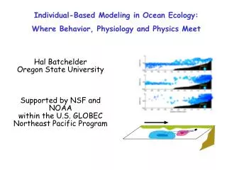
Individual-Based Modeling in Ocean Ecology: Where Behavior, Physiology and Physics Meet. Hal Batchelder Oregon State University Supported by NSF and NOAA within the U.S. GLOBEC Northeast Pacific Program. IBM Outline. Introduction to i-state distribution and i-state configuration models

E N D
Individual-Based Modeling in Ocean Ecology: Where Behavior, Physiology and Physics Meet Hal Batchelder Oregon State University Supported by NSF and NOAA within the U.S. GLOBEC Northeast Pacific Program
IBM Outline • Introduction to i-state distribution and i-state configuration models • How they differ • Why IBM’s • Advantages and Disadvantages • Eulerian-Lagrangian Coupled Approaches and Details • Examples • Design of Marine Protected Areas for Scallops • Nearshore retention (copepods in EBC upwelling regions; ADR) • DVM of dinoflagellates using a cell N quota model • Connectivity and Retention through Lagrangian Approaches • Considerations • Take Home Messages • Challenges and Opportunities
N P Z Ecosystem Model Franks et al., 1986
SOME BIOMASS Vitals: 380 lbs, 7’1”;
Vitals: ~380 lbs, Vitals: 380 lbs, 7’1”; MORE BIOMASS
? = Vitals: ~380 lbs, Vitals: 380 lbs, 7’1”;
? = Vitals: ~380 lbs, 40 mouths; Vitals: 380 lbs, 7’1”; one mouth; Actually able to put foot in mouth Regularly puts foot in mouth (figuratively)
Euphausia pacifica life stages N2 Metanauplius Calyptopi Adult
Individual Size • Impacts preferred prey type (abundance/size) • Impacts growth rate • Impacts mortality when size-dependent • Impacts behavior • Impacts internal pools (lipid reserves)
Euphausia pacifica life stages Stage-specific CW N2 Metanauplius ~7 μg ind-1 Calyptopi ~3.2 μg ind-1 Adult ~4000 μg ind-1
Euphausia pacifica life stages Stage-specific CW N2 Metanauplius ~7 μg ind-1 571 indiv. Calyptopi ~3.2 μg ind-1 1250 indiv. Adult ~4000 μg ind-1 1 indiv.
Allometric Relationships are Important Robin Ross (1982)
Allometric Relationships are Important (here it is weight specific relation) Robin Ross (1982)
Euphausia pacifica life stages Stage-specific CW ~7 μg ind-1 N2 Metanauplius 571 indiv. ΣR=529.2 ug C d-1 ΣG=519.6 ug C d-1 Calyptopi ~3.2 μg ind-1 1250 indiv. ΣR=633.6 ug C d-1 ΣG=425 ug C d-1 Adult ΣR=122.9 ug C d-1 ΣG=26 ug C d-1 ~4000 μg ind-1 1 indiv.
Body Size Prey Temperature Bioenergetics of an Individual Process R (ug C d-1) = f(Weight, Prey, Temp)
A Stage Progression Model E. pacifica Belehradek function for time to stage as function of temperature Basic Form is: Di = ai (T + b)c Di is the time (days) from egg to stage i ai is a stage specific constant b is a stage-independent shift in temperature c is assumed to be -2.05 (commonly observed from experiments; determines the curvature) Data from Ross (1982) and Feinberg et al. (2006) What if low food conditions delay development? Revised Form is: Di = [ai (T + b)c] / [1 – e-kP]
Interindividual variation in lipid weight of C5 stage of Calanus pacificus Laboratory reared individuals (range of hi to low food) varied by a factor of ca. 2.5; lipid content in field collected individuals even more variable (ca. 2.8) 2.8 2.5 Hakanson (1984, Limnol.Oceanog.)
i-state Distribution Models • fundamental tools of demographic theory • produce differential or difference equations • examples: • NPZ+ models • Lotka-Volterra predator-prey models • McKendrick-von Foerster equations • Suppose: • One population; two important dimensions control dynamics: individual age and individual size; given the assumption that all individuals experience the same environment (global mixing), then all individuals with the same i-state will have the same dynamics and can be treated collectively.
Suppose: Only indiv body size and life-stage are important to dynamics… Then: Could model population using n life-stages, each having mn wt classes. Life Stage Within Stage Weight What if: There are many more dimensions important to dynamics?
“It is impossible to predict the response of all but the very simplest natural systems from knowledge of current environmental stimuli alone. The problem is that the past of the system affects its response in the present.” Caswell and John (1992, p. 37) System State = f(History,Curr. Envir.) both are required to describe the systems behavior (deterministic) or probability distribution of systems behavior (stochastic)
Individual Size • Impacts preferred prey type (abundance/size) • Impacts growth rate • Impacts mortality when size-dependent • Impacts behavior Some early classic examples…
Intraspecific Effects - Initial Condition Sensitivity Interspecific Effects – Relative Size All figures are from Huston, M., D. DeAngelis, and W. Post. 1988. New computer models unify ecological theory. BioScience 38 (10), 682-691.
= f (history) • i-state configuration models • (aka Individual Based Models) • Each individual has a vector of characteristics associated with it • Examples are: • Body size (weight, length) • Age • Reproductive Condition • Nutritional (structural or physiological) Condition • Behavior • Location = Defines Present Environment
ZP • Conditions in which i-state distribution models are insufficient and i-state configuration models (IBMs) are necessary: • Complicated i-states – • Many elements in i-state configuration vector; numerical solutions as ‘distribution’ difficult • Small populations • Demographic analysis of endangered species • Viability of small populations • Local spatial interactions important • Spatial heterogeneity of the environment • Local interaction of individuals • Size- or individual-specific behaviors
Advantages of i-state configuration (IBMs) • Biology is often mechanistically explicit. (not hidden in differential equations). • Biological-Physical-Chemical Interactions are clearly detailed. • Individual is the fundamental biological unit, thus it is natural and intuitive to model at that level, rather than at the population level. • Allows explicit inclusion of an individual’s history and behavior. • History-Spatial Heterogeneity interactions ‘easily’ handled.
Costs Involved in IBM Approach • Difficult to implement feedback from IBM (Lagrangian) to underlying Eulerian model, esp. across multiple trophic levels • Consumption (depletion) of prey (E) by predators (L) • Assume not important (Batchelder & co. 1989,1995) • Conversion to concentrations per grid cell (Carlotti & Wolf 1998) • 2) Requirement for Large Numbers of Particles • Difficult to simulate realistic abundances • Each particle may represent one (IBM) or a variable number of identical individuals (Lag. Ens. Method/Superindividuals) • 3) Difficult (Impossible?) to simulate density dependence • 4) Extensive Computation Penalty • Biological/biochemical processes for individuals are many and complex • 5) Increased knowledge about the system (this might be a good thing)
Design of Marine Protected Areas The NW Atlantic Scallop Example
Scallop Larval Drift from Proposed Closed Regions Issues: larval repopulation of source regions, as well as non-closed regions; Long-term effects of marine protected areas
Retention effect of circulation over a single 40-day pelagic period within the fall climatology. • There is exchange between closed areas 1 and 2. • Area 1 is largely self-seeding; Area 2 seeds both areas. Source
10 Year Scallop Simulation w/ 1 spawning per year; 40 day larval drift; individual surviving scallops plotted (red are oldest individuals) No Closed Regions Closed Regions
Impacts of Dispersal Single, patchy Population (open) Metapopulation (structured connectance) Separate (closed) High Low Population Connectivity From C. Grant Law (unpubl.) Modified from Harrison and Taylor (1997)
Transport patterns From C. Grant Law (unpubl.)
How connected are different populations and does connectivity change with population structure or physical forcing? Are all populations equally valuable when protected? Do some regions act primarily as sources and others as sinks? How often is a given area dependent on recruits from elsewhere? Under which conditions is a given area self-seeding and how often are those conditions present? Are there regions of the coast that are particularly robust in terms of self seeding and which also act frequently as a source for remote areas? Questions Modified from C. Grant Law (unpubl.)
Management History Pre-Closure Distribution • NE side of Georges Bank • NE side of Nantucket shoals • Head of Hudson Canyon From C. Grant Law (unpubl.)
Management History Post-Closure Distribution • CLII north & south • CLI SW side of Georges Bank • NE side of Nantucket shoals • Head of Hudson Canyon • Poor recruitment in NLS and VBC closed areas From C. Grant Law (unpubl.)
Zooplankton Population Dynamics in 2D The Oregon Upwelling System
Spatially-Explicit Model Physical Exchange B, Predation T, B, , L Ingestion T, B, , L, P Egestion, P Age, Size, Number of Organisms Migration T, B, P Starvation T, B, P, Respiration T, B, Bioenergetic Model Processes and Environmental Variables Influencing Organism Growth and Number T = Temperature; B=Behavior; =Turbulence; P=Prey; L=Light
Physical Forcing (light,wind,IC's) Individual Zooplankton Characteristics (wt,stage,condition, sex, position) IBM with simulated Lagrangian Particles Eulerian Fields (velocity, temperature light, food, K) Population Characteristics (Demography) and Spatial Distribution 2D or 3D Eulerian Model Modeling Approach (Eulerian-Lagrangian Coupling)
Biological Organisms are not Passive Tracers Euphausia pacifica at NH25 (Aug 4, 2000, daytime) 0-10m 10-20m 20-50m Nauplii Calyptopes Depth Range of Layer Sampled 50-100m Furcilia All Stages are in upper 20 m during Night Juveniles 100-150m Adults 150-200m 0.0 5.0 10.0 15.0 20.0 25.0 30.0 35.0 Density (# m ) -3 Figure courtesy of J. Keister
Shelf Stations Slope Stations Life History Stage Life History Stage Calyptopis Calyptopis Juvenile Juvenile Adult Adult Egg Egg F1 F2 F3 F4 F6 F7 F1 F2 F3 F4 F6 F7 0 0 25 25 Depth (m) 50 50 75 75 Depth (m) 100 100 125 The top of the vertical bar represents the nighttime Average WMD. The bottom of the bar represents the daytime Average WMD. The height of the bar therefore represents the magnitude of DVM. 150 175 200 Magnitude of Diel Vertical Migration by Life Stage Based on 6 day-night paired MOCNESS From shelf stations and 8 day-night pairs From slope stations. Vance et al. (unpublished)
Individual Based Copepod Model (IBM) • Bioenergetics based model • dW/dt = Assimilation - Respiration • Growth is a function of weight, hunger condition, ambient food • Reproduction within C6 females with weight specific allocation between somatic and reproductive growth • Stage-specific, spatially-constant and weight-based mortality • Diel Vertical Migration behavior dependent on • light • size (weight) • hunger condition • food resources • proximity to boundaries 10 m during night 160 m during day Batchelder et al. (2002, PiO)
Batchelder and Williams (1995) Individual-based modelling of the population dynamics of Metridia lucens in the North Atlantic. ICES J. Mar. Sci., 52, 469-482.
~2X starved fed Runge, J. A. 1980. Effects of hunger and season on the feeding behavior of Calanus pacificus. Limnol. Oceanogr., 25, 134-145. Batchelder, H. P. 1986. Phytoplankton balance in the oceanic subarctic Pacific: grazing impact of Metridia pacifica. Mar. Ecol. Prog. Ser., 34, 213-225.
Size (S) Light Hunger (H) Food (P) Slows downmig Slows upmig Boundary (Ns,Nb) H Batchelder et al. (2002, PiO)
200 m 100 km Physical Model • Southward wind-stress forcing of 0.5 dyne/cm2, either constant or alternating on/off with 5 or 10 day intervals • 2d (x-z) Vertical slice • Time-dependent, hydrostatic, Boussinesq, Navier-Stokes • Finite difference • KPP mixing • Explicit mixing-length Bottom Boundary Layer • 500 < dx (m) < 1500 • 1.5 m < dz (m) < 3.7 • Topography for Newport, OR • Initialized w/ April climatology Batchelder et al. (2002, PiO)
N P Z 2D Upwelling Scenario Simulations Batchelder et al. (2002, PiO)
Few Nearshore No-DVM Simulation (PTM forced with Eulerian Concentrations of Prey, Velocities, and Kv) Recently layed clutches in hi food region Day 20 Weight loss below mixed layer Day 40 Starvation Mortality Day 80 Size of bubble is proportional to individual weight Batchelder et al. (2002, PiO)
DVM Simulation (PTM forced with Eulerian Concentrations of Prey, Velocities, and Kv) Large Individuals Inshore Middepth aggregation offshore Day 20 Nearshore reproduction and retention No reproduction & mortality loss offshore Day 40 Population nearshore only Day 80 Size of bubble is proportional to individual weight Batchelder et al. (2002, PiO)