RFQ Tuning Method last results
120 likes | 281 Vues
This document presents the latest results from the IPHI-SPL collaboration meeting held at CERN on April 28-29, 2003. It focuses on the tuning of Radio Frequency Quadrupoles (RFQ), discussing mechanical and electromagnetic tuning methods, resonance frequency analysis, and voltage profile adjustments. Key findings include techniques to achieve high accuracy and fast tuning through slug tuners and dipole rods, alongside spectral analysis of resonance frequencies. The study validates the mathematical formalism used for modeling and tuning, ensuring optimal performance of the RFQ.

RFQ Tuning Method last results
E N D
Presentation Transcript
RFQ Tuning Methodlast results IPHI-SPL collaboration meeting - CERN 28 & 29 /04/2003 CEA/DSM/DAPNIA/SACM
V [kV] 4. Closest dipole modes frequencies 3. Dipole components presence within the accelerating mode f +D - fQ = fQ - f -D |uS(z)/uQ(z)|< 10-2 |uT(z)/uQ(z)|< 10-2 z [m] What do we electromagnetically tune ? 1. Resonance Frequency fQ : 352.21 MHz 2. Accelerating voltage profile : Vp(z) |(uQ(z)-Vp(z))/Vp(z)|< 10-2
Mode S et T (ST) Mode Q distribution S Quadripole Mode S = [ -1/2, 0, 1/2, 0] Q = [ -1/2, 1/2, -1/2, 1/2] T = [ 0, -1/2, 0, 1/2] S dipoleModes focalisation Kpq = 352,2 MHz …
Central region End regions 1. Slug tuners 2. « dipole » rods 3. Plate thickness What do we mechanically tune ?
Diagnosis Treatment 1. Model 2. Test bench 5. Mathematical formalism What is the ideal RFQ ? e.l.m. parameters of the real RFQ e.l.m. parameters mechanical devices 1. Slug tuners Frequencies 2. Dipole rods Field distribution 3. End plates 3. Spectral analysis The tuning tools that we have developed 4. Cold-model Defaults real RFQ / ideal RFQ Fast tuning High accuracy
Coupled, inhomogeneous, 4-wire line equivalent circuit End regions Central region End regions Boundary conditions M = hermetian operator (tM=M) Eigen values (R+) = resonance frequencies fQi, fSj, fTk Our model & the associated spectral analysis d2U/dz2 – A U = - (/c)2 U Eigen functions (orthogonal basis) = { vQi(z), vSj(z), vTk(z) } voltage base functions Refer to : A. France, F. Simoens, “Theoretical Analysis of a Real-life RFQ Using a 4-Wire Line Model and the Spectral Theory of Differential Operators.”, EPAC2002 Conference (Paris), June 2002
Measurements Model 3d simulations 2 L2 C1 3 L1 L3 C3 L4 C4 4 Comparison measurements / model / 3d simulations Refer to :F. Simoens, A. France, O. Delferrière, “An Equivalent 4-Wire Line Theoretical Model of Real RFQ based on the Spectral Differential Theory”, CEA-SACLAY, LINAC Conference (Gyungju, Korea), August 2002
uS(z) [u.a.] fQ 0 350,62 MHz 1 352,18 MHz 2 352,22 MHz -9,2.10-2<uD/uQ<10,6.10-2 uQ(z) [u.a.] -6,4.10-2<(uQ-Vp)/Vp<3,4.10-2 -0,4.10-2<uD/uQ<0,4.10-2 uT(z) [u.a.] -0,2.10-2<(uQ-Vp)/Vp<0,2.10-2 Slug tuners : fast simultaneous convergence RFQ 2x1m Ref: F. Simoens, A. France, J. Gaiffier, “A New RFQ Model applied to the Longitudinal Tuning of a Segmented, Inhomogeneous RFQ with Highly Irregularly Spaced Tuners”, EPAC2002 Conference (Paris), June 2002
A new tuning criteria : ‘quadratic shift frequency’ Voltage profiles of the first dipole mode before dipole rods tuning after dipole rods tuning steep slopes straightened slopes Dipole rods length adjustment Matching of the equivalent end loads When df(n)real RFQ df(n)ideal RFQ Good correspondence between the measured andthe ‘ideal’ dipole mode frequencies Refer to : F. Simoens, A. France, “Tuning procedure of the 5 MeV IPHI RFQ”, CEA-SACLAY, LINAC Conference (Gyungju, Korea), August 2002
End region mismatch characterization : parameter = L x f [m.MHz] L = RFQ half-length f = (mismatched resonance freq.) - (nominal cut-off freq.) Nominal mid-position thickness Example of the IPHI RFQ cold-model end region adjustment range[-0,24 m.MHz , +0,33 m.MHz] End plate thickness adjustment 0 m.MHz Refer to : F. Simoens, A. France, “Tuning procedure of the 5 MeV IPHI RFQ”, CEA-SACLAY, LINAC Conference (Gyungju, Korea), August 2002
End #1 End #2 Slugs are moved at some distance of the end being tuned i.e. for end#1, in planes #6, 7 and 8 of segment #1 = set of different voltage excitations Spectral analysis Parameter extraction from measurements End plate thickness adjustment The nominal plate thickness is well-adjusted, Refer to : F. Simoens, A. France, “Tuning procedure of the 5 MeV IPHI RFQ”, CEA-SACLAY, LINAC Conference (Gyungju, Korea), August 2002
Conclusion • Last results • The agreement between measurements, 3d simulations and our model validates our mathematical formalism. • The tuning procedures of the different mechanical devices have been developed and experimentally validated. • In a 2-m long RFQ, we have achieved relative voltage error lower than 10-2 within 3 steps of slug tuners displacements. • For the dipole rods adjustments, a new practical tuning criteria has been introduced, that ensures the convergence of tuning. • The end region mismatch can be characterized from a set different voltage excitations and directly related to the end plate thickness. • Studies in progress • Chronology of the different tuning procedures in the context of the RFQ machining and assembling steps. • RF power coupling (iris / loop).