4.2. Budget constraint
4.2. Budget constraint. Definition: combinations of real income-leisure that the i can achieve Characteristics: Line “price takers” Slope = wage rate (w) Maximization of U:

4.2. Budget constraint
E N D
Presentation Transcript
4.2. Budget constraint • Definition: combinations of real income-leisure that the ican achieve • Characteristics: • Line “price takers” • Slope = wage rate (w) • Maximization of U: • Subjective or psychological preferences (IC) and objective or market preferences (BC) highestIC, tangent to BC • The individual and the market “are in agreement” • Wage rate = MRS tangency • Over and underemployment
4.2. IC, BC, & Max. of U • IC: all combinations of L-l desired by the i with U; subjective or psychological preferences slope MRS • BC: all combinations of L-l achievable at certain w; objective or market information slope w • Max. of U: IC & BC together tangency, same slope: MRS = w • Question: what happens if the slope of BC is steeper than that of the IC?
4.2. IC, BC, & Max. of U • What do individuals do when w goes up? • Answer: L up … or l up (and L down)? • Derivation of the supply of labor curve • “Backward-bending” changes from person to person • Again: incomeeffect and substitution effect • Substitution effect : ∆L due to ∆w with Y > 0 • Income effect : ∆L due to ∆Y with w < 0 (l: normal) • Total effect: depends on the “strength” of the other two
4.2. IC, BC, & Max. of U The reasoning behind “backward-bending”: with ∆w ∆BC substitution > income; but as t goes by, ∆w ∆BC substitution < income Supply curve: when leisure is abundant, how is the MRS? Different individual curves: men vs. women?

