Download
1 / 25
250 likes | 435 Vues
Hierarchical Bayesian Analysis of the Spiny Lobster Fishery in California. Brian Kinlan, Steve Gaines, Deborah McArdle, Katherine Emery UCSB. The Original Data – An Exceptionally Long Catch-Effort Time Series. Goals.

E N D
Hierarchical Bayesian Analysis of the Spiny Lobster Fishery in California Brian Kinlan, Steve Gaines, Deborah McArdle, Katherine Emery UCSB
The Original Data – An Exceptionally Long Catch-Effort Time Series
Goals • Estimate dynamics of lobster population (including recruits and sublegals) over history of fishery • Evaluate alternative models for population replenishment • Examine interactive effects of variation in effort, climate, and population dynamics over long time series • NEED: Model linking catch-effort time series to population dynamics
Methods Overview • Size-Structured State-Space Model • Length-Weight relationships used to link biomass catch data to abundance in underlying model • Development of priors on growth, mortality, and size structure • Implementation in WinBUGS, analysis in Matlab
Components of an Hierarchical Bayesian Model • Data • Likelihood model for data (Observation Error – assumed lognormal) • Process Model • Prior distributions for parameters • Logical links specifying functional form of deterministic relationships among parameters
Process Equations Abundance Ns,y=[Ns−1,y−1 * exp(−M) − Ca−1,y−1* exp(−0.5M)] * Gs,s-1,y N1,y=Ry Ry ~ LogNormal(μrecruits,σ2recruits) Catch log(CPUEy) = log(q) + log(Ny) Growth Ly=Ly-1+B0 exp(B1Ly-1)
Results • Posterior distributions of parameters summarized by their mean • Evaluation of Model Fit • Patterns emerging from model – stock-recruitment relationships, climate correlations
6 legal stock x 10 3 total including catch escapement 2.5 2 1.5 No. of Lobsters 1 0.5 0 1900 1920 1940 1960 1980 2000 Year
7 x 10 2 total stock(1-8) sublegal stock(1-3) legal stock(4-8) 1.8 reproductive stock(3-8) 1.6 1.4 1.2 No. of Lobsters 1 0.8 0.6 0.4 0.2 1900 1910 1920 1930 1940 1950 1960 1970 1980 1990 2000 Year
exploitation rate exploitation rate 1 0.8 0.6 Fraction Exploited 0.4 0.2 0 1900 1920 1940 1960 1980 2000 Year
weight of avg legal lobster (lbs) 3.2 3 2.8 2.6 2.4 2.2 Weight (Lbs) 2 1.8 1.6 1.4 1900 1920 1940 1960 1980 2000 Year
6 recruitment x 10 11 10 9 8 7 6 No. of Lobsters 5 4 3 2 1 1900 1920 1940 1960 1980 2000 Year
growth parameter 35 34 ) 1 - y 1 - 33 32 31 30 Asymptotic Growth Rate (mm indiv 29 28 27 1900 1920 1940 1960 1980 2000 Year
Comparison with simpler standard fisheries models • DeLury depletion model (abundance) • Shaeffer surplus production model (biomass) • Both assume constant r, K, q and fit unknown No; model estimated by least-squares or MLE
Y Bayesian total biomass Schaeffer biomass (7 outliers) Schaefer biomass (12 outliers) DeLury biomass Comparison with Standard Fisheries Models Biomass Comparison: Schaeffer, De Lury and Bayesian (1888-2005) 9000000 8000000 7000000 6000000 Y 5000000 4000000 3000000 2000000 1000000 0 1880 1900 1920 1940 1960 1980 2000 Year
Model Fit and Residuals • Model vs. Predicted Total Catch • Model vs. Predicted CPUE • Residuals – Effect of Constant Catchability Assumptions
5 Actual by Predicted Catch in Lbs x 10 12 Data Regression 1:1 Line 10 8 6 Catch(Lbs) Observed 4 2 0 0 2 4 6 8 10 12 Catch(Lbs) Model 5 x 10
Catch-Effort Model Fit (Test Constant q Assumption) 4 10 Data 2005 Regression 1:1 Line 3 10 1950 CPUE(Lbs/Trap) Observed Data Points Color Coded by Year 2 10 1895 1 10 1 2 3 10 10 10 Expected CPUE = q*N[y]*P(g|s)*exp(-M/2)
‘Empirical’ Stock-Recruitment Relationships • No assumptions or priors specifying a relationship between stock and recruitment were included in model • Recruitment was fit based on Catch, Effort, and the dynamic state equations • Does an ‘empirical’ relationship arise in the model fit?
Stock-Recruitment Relationship 10000000 9000000 8000000 7000000 6000000 5000000 4000000 Recruitment in Year Y (No. of lobsters) 3000000 2000000 500000 1000000 5000000 Reproductive Stock in Year Y-1 (No. of lobsters)
Recruits per Adult vs. No. of Adults 5.5 5 4.5 Recruits in Year Y per Adult in Year Y-1 4 3.5 3 2.5 2 1.5 0 1 2 3 4 5 6 6 x 10 No. of Adults in Year Y-1
Future Model Directions • allow time-dependency of catchability, time+size dependent mortality • additional growth, mortality, size info via priors • age-structured version with explicit modeling of cohort growth-in-length • ocean climate covariates • Spatial Model
Future Model Directions • Spatial Model • use regional (port-based) catch-effort data • compare alternative models of connectivity via larval movement and/or juvenile migration • will help clarify the population dynamic mechanism underlying the compensatory recruits-per-spawner relationship (pre- or post-dispersal density dependence)
Applications in Context of the Sustainable Fisheries Group • Evaluate forecast and hindcast scenarios of changing temporal (and spatial) patterns of effort • Incorporate process and observation uncertainty explicitly using bayesian posteriors • Assess value of information in this fishery