Module 2: Bayesian Hierarchical Models
Module 2: Bayesian Hierarchical Models. Francesca Dominici Michael Griswold The Johns Hopkins University Bloomberg School of Public Health. Key Points from yesterday. “Multi-level” Models: Have covariates from many levels and their interactions

Module 2: Bayesian Hierarchical Models
E N D
Presentation Transcript
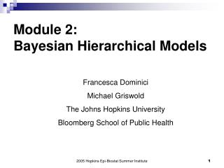
Module 2: Bayesian Hierarchical Models Francesca Dominici Michael Griswold The Johns Hopkins University Bloomberg School of Public Health 2005 Hopkins Epi-Biostat Summer Institute
Key Points from yesterday • “Multi-level” Models: • Have covariates from many levels and their interactions • Acknowledge correlation among observations from within a level (cluster) • Random effect MLMs condition on unobserved “latent variables” to describe correlations • Random Effects models fit naturally into a Bayesian paradigm • Bayesian methods combine prior beliefs with the likelihood of the observed data to obtain posterior inferences 2005 Hopkins Epi-Biostat Summer Institute
Bayesian Hierarchical Models • Module 2: • Example 1: School Test Scores • The simplest two-stage model • WinBUGS • Example 2: Aww Rats • A normal hierarchical model for repeated measures • WinBUGS 2005 Hopkins Epi-Biostat Summer Institute
Example 1: School Test Scores 2005 Hopkins Epi-Biostat Summer Institute
Testing in Schools • Goldstein et al. (1993) • Goal: differentiate between `good' and `bad‘ schools • Outcome: Standardized Test Scores • Sample: 1978 students from 38 schools • MLM: students (obs) within schools (cluster) • Possible Analyses: • Calculate each school’s observed average score • Calculate an overall average for all schools • Borrow strength across schools to improve individual school estimates 2005 Hopkins Epi-Biostat Summer Institute
Testing in Schools • Why borrow information across schools? • Median # of students per school: 48, Range: 1-198 • Suppose small school (N=3) has: 90, 90,10 (avg=63) • Suppose large school (N=100) has avg=65 • Suppose school with N=1 has: 69 (avg=69) • Which school is ‘better’? • Difficult to say, small N highly variable estimates • For larger schools we have good estimates, for smaller schools we may be able to borrow information from other schools to obtain more accurate estimates • How? Bayes 2005 Hopkins Epi-Biostat Summer Institute
Testing in Schools: “Direct Estimates” Mean Scores & C.I.s for Individual Schools Model: E(Yij) = j = + b*j b*j 2005 Hopkins Epi-Biostat Summer Institute
j= X(overall avg) j= Xj(shool avg) Fixed and Random Effects • Standard Normal regression models: ij ~ N(0,2) 1. Yij = + ij 2. Yij = j+ ij =+ b*j+ ij Fixed Effects = X + b*j = X + (Xj – X) 2005 Hopkins Epi-Biostat Summer Institute
j= X(overall avg) j= Xj(shool avg) Fixed and Random Effects • Standard Normal regression models: ij ~ N(0,2) 1. Yij = + ij 2. Yij = j+ ij =+ b*j+ ij • A random effects model: 3. Yij | bj = + bj+ ij, with: bj ~ N(0,2)Random Effects Fixed Effects = X + b*j = X + (Xj – X) Represents Prior beliefs about similarities between schools! 2005 Hopkins Epi-Biostat Summer Institute
j= X(overall avg) j= Xj(shool avg) j= X+ bjblup= X + b*j = X + (Xj – X) Fixed and Random Effects • Standard Normal regression models: ij ~ N(0,2) 1. Yij = + ij 2. Yij = j+ ij =+ b*j+ ij • A random effects model: 3. Yij | bj = + bj+ ij, with: bj ~ N(0,2)Random Effects • Estimate is part-way between the model and the data • Amount depends on variability () and underlying truth () Fixed Effects = X + b*j = X + (Xj – X) 2005 Hopkins Epi-Biostat Summer Institute
Testing in Schools: Shrinkage Plot b*j bj 2005 Hopkins Epi-Biostat Summer Institute
Testing in Schools: Winbugs • Data: i=1..1978 (students), s=1…38 (schools) • Model: • Yis ~ Normal(s , 2y) • s ~ Normal( , 2) (priors on school avgs) Note: WinBUGS uses precision instead of variance to specify a normal distribution! • WinBUGS: • Yis ~ Normal(s , y) with: 2y = 1 / y • s ~ Normal( , ) with: 2 = 1 / 2005 Hopkins Epi-Biostat Summer Institute
Testing in Schools: Winbugs • WinBUGS Model: • Yis ~ Normal(s , y) with: 2y = 1 / y • s ~ Normal( , ) with: 2 = 1 / • y ~ (0.001,0.001) (prior on precision) • Hyperpriors • Prior on mean of school means • ~ Normal(0 , 1/1000000) • Prior on precision (inv. variance) of school means • ~ (0.001,0.001) • Using “Vague” / “Noninformative” Priors 2005 Hopkins Epi-Biostat Summer Institute
Testing in Schools: Winbugs • Full WinBUGS Model: • Yis ~ Normal(s , y) with: 2y = 1 / y • s ~ Normal( , ) with: 2 = 1 / • y ~ (0.001,0.001) • ~ Normal(0 , 1/1000000) • ~ (0.001,0.001) 2005 Hopkins Epi-Biostat Summer Institute
Testing in Schools: Winbugs • WinBUGS Code: model { for( i in 1 : N ) { Y[i] ~ dnorm(mu[i],y.tau) mu[i] <- alpha[school[i]] } for( s in 1 : M ) { alpha[s] ~ dnorm(alpha.c, alpha.tau) } y.tau ~ dgamma(0.001,0.001) sigma <- 1 / sqrt(y.tau) alpha.c ~ dnorm(0.0,1.0E-6) alpha.tau ~ dgamma(0.001,0.001) } 2005 Hopkins Epi-Biostat Summer Institute
Example 2: Aww, Rats…A normal hierarchical model for repeated measures 2005 Hopkins Epi-Biostat Summer Institute
Improving individual-level estimates • Gelfand et al (1990) • 30 young rats, weights measured weekly for five weeks • Dependent variable (Yij) is weight for rat “i” at week “j” • Data: • Multilevel: weights (observations) within rats (clusters) 2005 Hopkins Epi-Biostat Summer Institute
Individual & population growth • Rat “i” has its own expected growth line: E(Yij) = b0i + b1iXj • There is also an overall, average population growth line: E(Yij) = 0 + 1Xj Weight Pop line (average growth) Individual Growth Lines Study Day (centered) 2005 Hopkins Epi-Biostat Summer Institute
Improving individual-level estimates • Possible Analyses • Each rat (cluster) has its own line: intercept= bi0, slope= bi1 • All rats follow the same line: bi0 = 0, bi1 = 1 • A compromise between these two: Each rat has its own line, BUT… the lines come from an assumed distribution E(Yij | bi0, bi1) = bi0 + bi1Xj bi0 ~ N(0, 02) bi1 ~ N(1, 12) “Random Effects” 2005 Hopkins Epi-Biostat Summer Institute
A compromise: Each rat has its own line, but information is borrowed across rats to tell us about individual rat growth Weight Pop line (average growth) Bayes-Shrunk Individual Growth Lines 2005 Hopkins Epi-Biostat Summer Institute Study Day (centered)
Rats: Winbugs (see help: Examples Vol I) • WinBUGS Model: 2005 Hopkins Epi-Biostat Summer Institute
Rats: Winbugs (see help: Examples Vol I) • WinBUGS Code: 2005 Hopkins Epi-Biostat Summer Institute
Rats: Winbugs (see help: Examples Vol I) • WinBUGS Results: 10000 updates 2005 Hopkins Epi-Biostat Summer Institute
WinBUGS Diagnostics: • MC error tells you to what extent simulation error contributes to the uncertainty in the estimation of the mean. • This can be reduced by generating additional samples. • Always examine the trace of the samples. • To do this select the history button on the Sample Monitor Tool. • Look for: • Trends • Correlations 2005 Hopkins Epi-Biostat Summer Institute
Rats: Winbugs (see help: Examples Vol I) • WinBUGS Diagnostics: history 2005 Hopkins Epi-Biostat Summer Institute
WinBUGS Diagnostics: • Examine sample autocorrelation directly by selecting the ‘auto cor’ button. • If autocorrelation exists, generate additional samples and thin more. 2005 Hopkins Epi-Biostat Summer Institute
Rats: Winbugs (see help: Examples Vol I) • WinBUGS Diagnostics: autocorrelation 2005 Hopkins Epi-Biostat Summer Institute
WinBUGS provides machinery for Bayesian paradigm “shrinkage estimates” in MLMs Bayes Weight Weight Pop line (average growth) Pop line (average growth) Bayes-Shrunk Growth Lines Individual Growth Lines Study Day (centered) 2005 Hopkins Epi-Biostat Summer Institute Study Day (centered)
School Test Scores Revisited 2005 Hopkins Epi-Biostat Summer Institute
Testing in Schools revisited • Suppose we wanted to include covariate information in the school test scores example • Student-level covariates • Gender • London Reading Test (LRT) score • Verbal reasoning (VR) test category (1, 2 or 3) • School -level covariates • Gender intake (all girls, all boys or mixed) • Religious denomination (Church of England, Roman Catholic, State school or other) 2005 Hopkins Epi-Biostat Summer Institute
Testing in Schools revisited • Model • Wow! Can YOU fit this model? • Yes you can! • See WinBUGS>help>Examples Vol II for data, code, results, etc. • More Importantly: Do you understand this model? 2005 Hopkins Epi-Biostat Summer Institute
Bayesian Concepts • Frequentist: Parameters are “the truth” • Bayesian: Parameters have a distribution • “Borrow Strength” from other observations • “Shrink Estimates” towards overall averages • Compromise between model & data • Incorporate prior/other information in estimates • Account for other sources of uncertainty • Posterior Likelihood * Prior 2005 Hopkins Epi-Biostat Summer Institute