Spatial Data Analysis
Spatial Data Analysis. GROUP MEMBERS KAVIVENTHAN A/L VISUVANATHAN THAMIL VAANI A/P KRISHNAN TEE SENG TECK TANG LI WAH KHAIRUL ARIFFIN SUIB SITI SHAHHIDA ABDULLAH NUR AIN ABD HAKAM. Spatial analysis.

Spatial Data Analysis
E N D
Presentation Transcript
Spatial Data Analysis • GROUP MEMBERS • KAVIVENTHAN A/L VISUVANATHAN • THAMIL VAANI A/P KRISHNAN • TEE SENG TECK • TANG LI WAH • KHAIRUL ARIFFIN SUIB • SITI SHAHHIDA ABDULLAH • NUR AIN ABD HAKAM
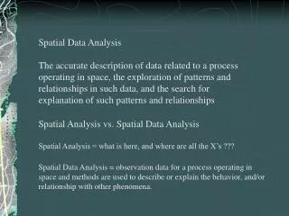
Spatial analysis Spatial analysis is the vital part of GIS. Spatial analysis in GIS involves three types of operations • attribute query (also known as non-spatial), • spatial query • and generation of new data sets from the original databases.
Spatial Data Analysis • Representation of reality • Purpose is to understand, describe, predict the real world scenarios • Gives a simplified , manageable view of the real world
Attribute Query ArcView’s Query Builder ([State name] = “California” or “New York”) ([City name] = “San*”) New Set Add to Set Select from Set Command line Query (Arc/Info) find in states where state_name = ‘California’ <1 record in result> calculate in states population_density = population / area <50 records in result> restrict in states where population_density > 1000 <20 records selected in result>>
Attribute Query Using Boolean Logic • Data retrieval is done by applying the rules of Boolean logic to operate on the attributes. • Boolean algebra uses the operators AND, OR, XOR and NOT to see whether a particular condition is true or not. • Ex. TYPE = ‘ASPHALT’ AND LENGTH = 4000 AND LANES = 4 • Simple Boolean logic is often portrayed visually in the form of Venn diagrams
VENN DIAGRAM A AND B = Result T T T T F F F T F F F F B A B A A AND B A NOT B A XOR B = Result T T F T F T F T T F F F A OR B = Result T T T T F T F T T F F F A A B B A OR B A XOR B B B A A C C (A AND B) OR C A AND (B OR C)
Spatial Search/Query • Overlay is a spatial retrieval operation that is equivalent to an attribute join. • Buffering is a spatial retrieval around points, lines, or areas based on distance.
Find all houses within a certain area that have tiled roofs and five bedrooms, then list their characteristics.
Buffering • can be constructed around a point, line or area. • Buffering algorithm creates a new area enclosing the buffered object. • The applications of this buffering operations include, for example, identifying protected zone around lakes and streams, zone of noise pollution around highways, service zone around bus route, or groundwater pollution zone around waste site.
Spatial Overlay • An operation that merges the features of two coverage layers into a new layer and relationally joins their feature attribute table. • When overlay occurs, spatial relationships between objects are updated for the new, combined map. • In some circumstances, the result may be information about relationships (new attributes) for the old maps rather than the creation of new objects.
GIS usage in Spatial Analysis GIS operational procedure and analytical task that are particularly useful for spatial analysis • Single layer operations • Multi layer operations/ Topological overlay • Spatial modeling • Geometric modeling • Calculating the distance between geographic features • Calculating area, length and perimeter • Geometric buffers. • Point pattern analysis • Network analysis • Surface analysis • Raster/Grid analysis • Fuzzy Spatial Analysis • Geostatistical Tools for Spatial Analysis
Point pattern analysis • It deals with the examination and evaluation of spatial patterns and the processes of point features. • Distribution of an endangered species examined in a point pattern analysis
Vector Based Spatial Data Analysis • There are multi layer operations, which allow combining features from different layers to form a new map and give new information and features that were not present in the individual maps. • Topological overlays: Selective overlay of polygons, lines and points enables the users to generate a map containing features and attributes of interest, extracted from different themes or layers.
Topological overlays Point-in-polygon overlay • Point-in-polygon algorithm overlays point objects on areas and compute "is contained in" relationship. • The result is a new attribute for each point specifying the polygon it belongs to. Map overlay - point in polygon
Line-on-Polygon Overlay • Line-on-polygon algorithm overlays line objects on area objects and compute "is contained in" relationship. • Lines are broken at each area object boundary to form new line segments and new attributes created for each output line specifying the area it belongs to.
Polygon-on-Polygon Overlay • Polygon-on-polygon algorithm overlay two layers of area objects. • Boundaries of polygons are broken at each intersection and new areas are created. • During polygon overlay, many new and smaller polygons may be created, some of which may not represent true spatial variations.
Network analysis: • Designed specifically for line features organized in connected networks, typically applies to transportation problems and location analysis such as school bus routing, passenger plotting, walking distance, bus stop optimization, optimum path finding etc.
Surface analysis • Deals with the spatial distribution of surface information in terms of a three-dimensional structure. • The distribution of any spatial phenomenon can be displayed in a three dimensional perspective diagram for visual examination.
Grid analysis • Involves the processing of spatial data in a special, regularly spaced form. The following illustration shows a grid-based model of fire progression. The darkest cells in the grid represent the area where a fire is currently underway.
Geostatistical Tools For Spatial Analysis Geostatistics studies spatial variability of regionalized variables: Variables that have an attribute value and a location in a two or three- dimensional space.
Tools to characterize the spatial variability are: 1)Spatial Autocorrelation Function • statistics measure and analyze the degree of dependency among observations in a geographic space. • Classic spatial autocorrelation statistics include Moran's I and Geary's C.
2)Semivariogram • The semivariogram functions quantifies the assumption that things nearby tend to be more similar than things that are farther apart. • Semivariogram measures the strength of statistical correlation as a function of distance.
Types of semivariogram models • Geostatistical Analyst provides the following functions to choose from to model the empirical semivariogram: • Circular • Spherical • Tetraspherical • Pentaspherical • Exponential • Gaussian • Rational Quadratic • Hole Effect • K-Bessel • J-Bessel • Stable
INTERPOLATION • Method to estimate variables based on values at observed locations. • Assumption • The influence of one known point over an unknown point increases as distance between them decreases. • 4 methods included:
a) Inverse distance weighting - reduce the variable with decreasing nearness from observed location b) Kriging method -interpolates space according to spatial lag relationship with both systematic & random components c)Thiessenmehod d)Spline method
Accuracy of Interpolation • Depends on accuracy, number and distribution of the known points used in the calculation • Depends on how accurate the mathematical function used correctly models the phenomenon. As the assumptions of the model are more severely violated, the interpolation results become less accurate. • No matter which interpolator is selected, the more input points and the greater their distribution, the more reliable the results.
Raster Based Spatial Data Analysis • A raster is a GIS data structure comprised of a matrix of rectangular grid cells. • Each cell represents a specific area on the ground. • Resolution of raster is defined by the ground area represented by the raster grid cell. • The higher the resolution of the grid, the more cells are required to portray a given area of ground surface.
The resolution of raster is often a function of the scale of the map from which the spatial data may have been scanned or digitized. • In raster analysis, geographic units are regularly spaced and the location of each unit is referenced by row & column positions. • Because geographic units are of equal size & identical shape, area adjustment of geographic units is unnecessary & spatial properties of geographic entities are relatively easy to trace
Advantages of using the Raster Format in Spatial Analysis • Efficient processing: Because geographic units are regularly spaced with identical spatial properties, multiple layer operations can be processed very efficiently. • Numerous existing sources: Grids are the common format for numerous sources of spatial information including satellite imagery, scanned aerial photos, and digital elevation models, among others. • Different feature types organized in the same layer: For instance, the same grid may consist of point features, line features, and area features, as long as different features are assigned different values
Raster Overlay Replace all 0’s in B with data from A A B
Pixels • A term employed in the field of remote sensing. • Like grid cell, portray an area subdivided into very small square cells. • The result of capturing data through the digitization of aerial/satellite imagery. • Image resolution is stated by defining the ground area represented by one pixel. • Identified by unique numerical codes called a digital number. • Each cell has only one digital number.
Grid Format Disadvantages • Data redundancy: When data elements are organized in a regularly spaced system, there is a data point at the location of every grid cell, regardless of whether the data element is needed or not. • Resolution confusion: Gridded data give an unnatural look and unrealistic presentation unless the resolution is sufficiently high. Conversely , spatial resolution dictates spatial properties. For instance, some spatial statistics derived from a distribution may be different, if spatial resolution varies, which is the result of the well-known scale problem. • Cell value assignment difficulties: Different methods of cell value assignment may result in quite different spatial patterns.
Reclassification • Reclassification is to reassign new thematic values or codes to units of spatial feature, which will result in merging polygons. • A set of "reclassify attributes", "dissolve the boundaries" and "merge the polygons" are used frequently in aggregating area objects
Grid Operations used in Map Algebra Map Algebra performs following four basic operations: • Local functions: that work on every single cell, • Focal functions: that process the data of each cell based on the information of a specified neighborhood, • Zonal functions: that provide operations that work on each group of cells of identical values, and • Global functions: that work on a cell based on the data of the entire
Local Function Focal Function Global Function Grid operations Zonal Function
Some important raster analysis operations • Renumbering areas in a grid file • Characterizing Terrain Feature • Performing a Cost surface analysis • Performing on Optimal Path analysis • Performing proximity Search • Creating Variable-Width Buffers
Classification A-B : agriculture soil C-E : non agriculture soil Soil map Agricultural soil map -Altering attribute values without changing geometry. -to see new pattern and connection
Characterizing Terrain Feature • Identifying Convex and Concave features by deviation from the trend of the terrain. Figures from Asia Asian Institute of Technology Source:Lecture notes from the Asian Institute of Technology
Characterizing Terrain Feature • 2-D, 3-D and draped displays of terrain slope Figures from Asia Asian Institute of Technology Source:Lecture notes from the Asian Institute of Technology
Routing and Optimal Paths The steepest downhill path from the Substation over the Accumulated Cost surface identifies the Most referred Route minimizing visual exposure to houses. Figures from Asia Asian Institute of Technology Source:Lecture Notes from Asian Institute of Technology
Routing and Optimal Paths Alternate routes are generated by evaluating the model using weights derived from different group perspectives Figures from Asia Asian Institute of Technology Source:Lecture notes from the Asian Institute of Technology