Download
1 / 20
210 likes | 248 Vues
Learn about image restoration techniques such as inverse filtering and Wiener filtering, along with morphological processing like dilation and erosion. Practice coding examples in MATLAB.

E N D
Image Restoration II& Morphological Processing Comp344 Tutorial Kai Zhang
Outline • Imgae Degradation Model • Inverse Filter • Wiener Filter • Morphological Processing
Degradation Model • Spatial domain • Frequency domain • Problem Definition • Observe the degraded image g(x,y) • H function and N (noise) are either known or need to be estimated • Goal: restore the original image f(x,y)
H can be obtained by • Observing the image (say, blurred) • Modeling, example: • atmospheric turbulence: • Motion blur:
Inverse Filtering • Simple (noiseless) case: • Then original image can be obtained by • Note: H(u,v) may have many small entries (close to 0) that spoil the result. • Restrict the area to low frequency part or use Gaussian weighting to solve this problem.
Wiener Filtering • Noise can be handled explicitly • In case there is no noise, this is inverse filtering • When noise is difficult to estimate, simply replace the power spectrum ratio between image and noise with a constant K
Functions • Matlab builtin functions • PSF = fspecial(‘type’, paras); • All kinds of spatial filters. Type includes ‘average’, ‘disk’, ‘gaussian’,’motion’… • Paras are corresponding parameters • PSF is the spatial domain filter created • Type help fspecial for more • fr = deconvwnr(g, PSF, NSPR); • Wiener filrering. G is corrupted image, fr is restored one • PSF is the filter that degrades the image • NSPR: noise to signal power ratio • Type help deconvwnr for more
Example (noiseless) • Inverse filtering
Codes • f = checkerboard(20); • figure, imshow(f,[]); xlabel('original image') • PSF = fspecial('motion',7,45); • gb = imfilter(f,PSF,'circular'); • figure, imshow(gb,[]); xlabel('motion blurred') • fr = deconvwnr(gb,PSF); • figure, imshow(fr,[]);xlabel('restored');
Codes • f = checkerboard(8); • PSF = fspecial('motion',7,45); • gb = imfilter(f,PSF,'circular'); • noise = normrnd(0,0.001^0.5,size(f)); • gb = gb + noise; • figure,subplot(1,3,1);imshow(gb,[]); xlabel('noisy image'); • fr1 = deconvwnr(gb, PSF); • subplot(1,3,2),imshow(fr1,[]); xlabel('inverse filtering'); • Sn = abs(fft2(noise)).^2; %noise power spectrum • nA = mean(Sn(:)); % noise average power; • Sf = abs(fft2(f)).^2; %image power spectrum • fA = mean(Sf(:)); %image average spectrum • R = nA/fA; • fr2 = deconvwnr(gb,PSF,R); • subplot(1,3,3); imshow(fr2,[]);xlabel('Wiener filtering');
Image dilation and Erosion, opening and closing • For binary images, after specifying a structuring element: • Dilation: grows or thickens the object • Erosion: shrinks or thins object • Opening of A by B, is simply erosion of A by B, followed by dilation of the result by B. • Closing of A by B, is dilation followed by erosion (opposite to opening).
Codes • A = imread('broken-text.tif'); • B = [0 1 0; 1 1 1; 0 1 0]; • A2 = imdilate(A,B); • imshow(A) • figure,imshow(A)
Codes • A = imread('mask.tif'); • figure,imshow(A); • se = strel('disk',10); • A2 = imerode(A, se); • figure,imshow(A2); • se = strel('disk',5); • A3 = imerode(A, se); • figure,imshow(A3); • se = strel('disk',20); • A4 = imerode(A, se); • figure,imshow(A4);
Opening and Closing • Original image; opening • Closing; closing of top right image
f = imread('shapes.tif'); • figure,imshow(f); • se = strel('square', 20); • fo = imopen(f, se); • figure,imshow(fo); • fc = imclose(f, se); • figure,imshow(fc) • foc = imclose(fo,se); • figure,imshow(foc);
Codes • f = imread('noisy-fingerprint.tif'); • figure,imshow(f); • se = strel('square', 3); • fo = imopen(f,se); • figure,imshow(fo); • foc = imclose(fo,se); • figure,imshow(foc);