Phase Equilibrium
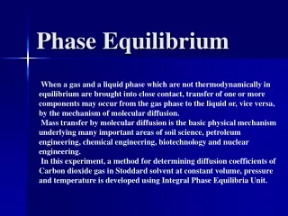
Phase Equilibrium. When a gas and a liquid phase which are not thermodynamically in equilibrium are brought into close contact, transfer of one or more components may occur from the gas phase to the liquid or, vice versa, by the mechanism of molecular diffusion.

Phase Equilibrium
E N D
Presentation Transcript
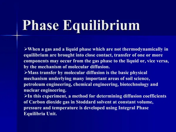
Phase Equilibrium • When a gas and a liquid phase which are not thermodynamically in equilibrium are brought into close contact, transfer of one or more components may occur from the gas phase to the liquid or, vice versa, by the mechanism of molecular diffusion. • Mass transfer by molecular diffusion is the basic physical mechanism underlying many important areas of soil science, petroleum engineering, chemical engineering, biotechnology and nuclear engineering. • In this experiment, a method for determining diffusion coefficients of Carbon dioxide gas in Stoddard solvent at constant volume, pressure and temperature is developed using Integral Phase Equilibria Unit.
Objective • Determine • diffusion coefficient, • Solubility, • Henrys Constant • The enthalpy of solution of carbon dioxide in Stoddard solvent in the range of 18 - 35°C and at 1.0 atmosphere pressure.
Introduction • Diffusion Coefficient • Measures the rate of diffusion • Time-dependent • Solubility • Measures maximum amount of gas dissolved in liquid • Time-independent • Henry’s Law constant • Dissolved gas in liquid is proportional to partial pressure in vapor phase • Heat of mixing • Correlation between Henry’s Law constant and T
Determination of diffusion coefficient from experimental data A number of mathematical models have been proposed to determine the diffusion coefficients from experimental volume–time profiles, however all these models are developed from the equation of continuity for the solute component: Gas phase C Cav where r = Rate of reaction (kg/m3s) J = Mass transfer by the mechanism of molecular diffusion (kg/m2s) v = Molar volume (m3) Interface Z Z(t) Z=0
Referring to Fig 1&2 • for a one-dimensional diffusion cell • absence of chemical reaction, • movement of the interface in the boundary conditions of the system, in which a component in the gas phase is absorbed into a liquid phase starting at time zero and continuing at longer times. Based upon a model proposed by Higbie (penetration theory) • the liquid interface is thus always at saturation, since the molecules can diffuse in the liquid phase away from the interface only at rates which are extremely low with respect to the rate at which gaseous molecules can be added to the interface. • It is also assumed that the distance between the interface and the bottom of the cell is semi-infinite; that is, diffusion is slow enough that the concentration at the bottom of the cell is negligible compared to the concentration at the interface. According to the film theory • the gas and the liquid phases at the interface are thermodynamically in equilibrium, i.e. the interface concentration of the solute, Ci remains unchanged as long as temperature and pressure of the system are kept constant. Gas V=104 CC Ci Stoddard Solvent V=100 CC Z(t) C(t,Z) Z
where C = Concentration of dissolved CO2 in the liquid phase at Z and t. Z = Distance in cm traveled from the liquid interface. t = time D12 =Diffusion coefficient of species 1 in 2. • Thus the unsteady-state differential equation representing concentration changes with time and position is: • Solution of Fick’s 2nd Law using the boundary conditions described is: • Solve for the number of moles added up to a time t: • If one plots NT versus t1/2, the slope of this line is equal to • 2ACi (D12/)1/2 The boundary conditions are: Z = 0 C = Ci Z ∞: C = 0 The initial condition is C = 0 at t = 0:
SolubilityHenry’s Law constant • The solubility of a gas in a liquid solvent may be represented to good accuracy at dilute concentrations of the dissolved gas by Henry's Law: f = H X • where f is the fugacity of the gas in the gas phase in equilibrium with the liquid phase of concentration X of dissolved gas. • H is the Henry’s law constant, which is a function of temperature. • Thus, by measuring the solubility one can obtain an estimate of the Henry's law constant.
n = gram moles of carbon dioxide absorbed in the liquid phase PT = corrected barometer reading = vapor pressure of Stoddard Solvent at cell temperature Tp = temperature at the pump Tc = temperature of the cell (bath temperature) = total gas volume delivered from the pump to the cell Vcg = volume of the gas phase in the cell Zp = compressibility factor of CO2 at pump T and PT Zc = compressibility factor of CO2 at cell T and PT Vd = dead volume in the system (cc)
The fugacity, f, can be determined from the Lewis and Randall Rule, which gives • f = fugacity of CO2 in the gas phase • fo = fugacity of pure gaseous CO2 at PT and cell T • y = mole fraction of CO2 in gas phase • Thus • by definition: • the fugacity coefficient for pure CO2 in the gas phase at cell T and P T
Heat of Mixing • Use Henry’s Law coefficients at the three experimental temperatures to obtain the heat of mixing: • Plotting ln(H) vs. 1/T gives a line with a slope of ΔHmix/R. • ΔHmix is expected to be negative, which would indicate that CO2 and Stoddard solvent are more energetically stable than apart (i.e., the interactions are favorable).
- Experimental: Cell Evacuation
- Experimental: Filling Syringe
+ Experimental: Reduce to Atmospheric Pressure
0 Experimental: Fill Cell between V4 and the cell is 40.5 cm and the pipe diameter is 0.15 cm
References • Koretsky, Milo D. Engineering and Chemical Thermodynamics. John Wiley & Sons, Inc., 2004. • Ophardt, Charles E. Virtual Chembook. Elmhurst College, 2003. [Online] Available at: http://www.elmhurst.edu/~chm/vchembook/174temppres.html • http://en.wikipedia.org/wiki/Lake_Nyos
Cell information • the dimension • Diameter = 51.43 mm • Height of the lid = 21.7 mm • Diameter to the lower section = 50.4 mm • Depth of the lower section averaged = 70.5 mm • Volume of the Stoddard liquid 100ml • Volume of the space (Gas) 104 ml