CHS 221 Visualizing Data
CHS 221 Visualizing Data. Week 3 Dr. Wajed Hatamleh http://staff.ksu.edu.sa/whatamleh/en. Visualizing Data. Depict the nature of shape or shape of the data distribution In a graph: Different graphs used for different types of data. Histogram. Another common graphical presentation of

CHS 221 Visualizing Data
E N D
Presentation Transcript
CHS 221Visualizing Data Week 3 Dr. WajedHatamleh http://staff.ksu.edu.sa/whatamleh/en
Visualizing Data • Depict the nature of shape or shape of the data distribution • In a graph: Different graphs used for different types of data
Histogram • Another common graphical presentation of quantitative data is a histogram. • The variable of interest is placed on the horizontal axis. • A rectangle is drawn above each class interval with • its height corresponding to the interval’s frequency, • relative frequency, or percent frequency.
Histograms • Histograms: Used for quantitative data • Similar to a bar graph, with an X and Y axis—but adjacent values are on a continuum so bars touch one another • Data values on X axis are arranged from lowest to highest • Bars are drawn to height to show frequency or percentage (Y axis)
Histograms (cont’d) • Example of a histogram: Heart rate data f Heart rate in bpm
Figure 2-1 Histogram A bar graph in which the horizontal scale represents the classes of data values and the vertical scale represents the frequencies.
Figure 2-2 Relative Frequency Histogram Has the same shape and horizontal scale as a histogram, but the vertical scale is marked with relative frequencies.
Histogram and Relative Frequency Histogram Figure 2-1 Figure 2-2
Ogive • An ogive is a graph of a cumulative distribution. • The data values are shown on the horizontal axis. • Shown on the vertical axis are the: • cumulative frequencies, or • cumulative relative frequencies, or • cumulative percent frequencies • The frequency (one of the above) of each class is plotted as a point. • The plotted points are connected by straight lines.
Figure 2-4 Ogive A line graph that depicts cumulative frequencies
Bar Graphs • Bar graphs: Used qualitative data. • Bar graphs have a horizontal dimension (X axis) that specifies categories (i.e., data values) • The vertical dimension (Y axis) specifies either frequencies or percentages • Bars for each category drawn to the height that indicates the frequency or %
Bar Graphs • Example of a bar graph • Note the bars do not touch each other
Pie Chart • Pie Charts: Also used for qualitative data. • Circle is divided into pie-shaped wedges corresponding to percentages for a given category or data value • All pieces add up to 100% • Place wedges in order, with biggest wedge starting at “12 o’clock”
Pie Chart • Example of a pie chart, for same marital status data
Recap In this Section we have discussed graphs that are pictures of distributions. Keep in mind that the object of this section is not just to construct graphs, but to learn something about the data sets – that is, to understand the nature of their distributions.
Characteristics of a Data Distribution • Central tendency • Variability • Both central tendency and variability can be expressed by indexes that are descriptive statistics
Central Tendency • Indexes of central tendency provide a single number to characterize a distribution • Measures of central tendency come from the center of the distribution of data values, indicating what is “typical,” and where data values tend to cluster • Popularly called an “average”
Central Tendency Indexes • Three alternative indexes: • The mode • The median • The mean
The mode is the score value with the highest frequency; the most “popular” score Age: 26 27 27 28 29 30 31 Mode = 27 The mode The Mode
The Mode: Advantages • Can be used with data measured on any measurement level (including nominal level) • Easy to “compute” • Reflects an actual value in the distribution, so it is easy to understand • Useful when there are 2+ “popular” scores (i.e., in multimodal distributions)
Mode A data set may be: Bimodal Multimodal No Mode • denoted by M • the only measure of central tendency that can be used with qualitative data
Examples • Mode is 1.10 • Bimodal - 27 & 55 • No Mode a. 5.40 1.10 0.42 0.73 0.48 1.10 b. 27 27 27 55 55 55 88 88 99 c. 1 2 3 6 7 8 9 10
The Mode: Disadvantages • Ignores most information in the distribution • Tends to be unstable (i.e., value varies a lot from one sample to the next) • Some distributions may not have a mode (e.g., 10, 10, 11, 11, 12, 12)
The median is the score that divides the distribution into two equal halves 50% are below the median, 50% above Age: 26 27 27 28 29 30 31 Median (Mdn) = 28 The median The Median
5.40 1.10 0.42 0.73 0.48 1.10 0.66 0.42 0.48 0.66 0.73 1.10 1.10 5.40 (in order - odd number of values) exact middle MEDIANis 0.73 5.40 1.10 0.42 0.73 0.48 1.10 0.42 0.48 0.73 1.10 1.10 5.40 (even number of values – no exact middle shared by two numbers) 0.73 + 1.10 MEDIAN is 0.915 2
The Median: Advantages • Not influenced by outliers • Particularly good index of what is “typical” when distribution is skewed • Easy to “compute”
The Median: Disadvantages • Does not take actual data values into account—only an index of position • Value of median not necessarily an actual data value, so it is more difficult to understand than mode
The mean is the arithmetic average Data values are summed and divided by N Age: 26 27 27 28 29 30 31 Mean = 28.3 The mean The Mean
The Mean (cont’d) • Most frequently used measure of central tendency • Equation: M = ΣX ÷ N • Where: M = sample mean Σ = the sum of X = actual data values N = number of people
The Mean: Advantages • The balance point in the distribution: • Sum of deviations above the mean always exactly balances those below it • Does not ignore any information • The most stable index of central tendency • Many inferential statistics are based on the mean
The Mean: Disadvantages • Sensitive to outliers • Gives a distorted view of what is “typical” when data are skewed • Value of mean is often not an actual data value
The Mean: Symbols • Sample means: • In reports, usually symbolized as M • In statistical formulas, usually symbolized as (pronounced X bar) • Population means: • The Greek letter μ (mu)
x is pronounced ‘x-bar’ and denotes the mean of a set of sample values ∑x x = n ∑x µ = N Notation µis pronounced ‘mu’ and denotes themean of all values in a population
Definitions • Symmetric Data is symmetric if the left half of its histogram is roughly a mirror image of its right half. • Skewed Data is skewed if it is not symmetric and if it extends more to one side than the other.
Figure 2-11 Skewness
Types of Measures of Center Mean Median Mode • Mean from a frequency distribution • Best Measures of Center • Skewness Recap In this section we have discussed:
Measures of Variation Because this section introduces the concept of variation, this is one of the most important sections in the entire book
lowest highest value value Definition The range of a set of data is the difference between the highest value and the lowest value
Definition The standard deviation of a set of sample values is a measure of variation of values about the mean
∑(x - x)2 S= n -1 Sample Standard Deviation Formula
n (∑x2)- (∑x)2 s = n (n -1) Sample Standard Deviation (Shortcut Formula)
Standard Deviation - Key Points • The standard deviation is a measure of variation of all values from the mean • The value of the standard deviation s is usually positive • The value of the standard deviation s can increase dramatically with the inclusion of one or more outliers (data values far away from all others) • The units of the standard deviation s are the same as the units of the original data values
Definition • Empirical (68-95-99.7) Rule For data sets having a distribution that is approximately bell shaped, the following properties apply: • About 68% of all values fall within 1 standard deviation of the mean • About 95% of all values fall within 2 standard deviations of the mean • About 99.7% of all values fall within 3 standard deviations of the mean
The Empirical Rule FIGURE 2-13
The Empirical Rule FIGURE 2-13
The Empirical Rule FIGURE 2-13
Are you Ready • Post test Time
Which measure of center is the only one that can be used with data at the catogrical level of measurement? • Mean • Median • Mode
Which of the following measures of center is not affected by outliers? • Mean • Median • Mode